Download
1 / 28
280 likes | 338 Vues
Explore the complex framework of the Mundell-Fleming model in open economies, analyzing the impacts of fiscal and monetary policies, exchange rate mechanisms, and trade protectionism. Learn about the effectiveness of policy interventions and the influence of political risk on economic outcomes.

E N D
The Mundell-Fleming Model • Assumption • Small open economy • Free capital mobility (r = r*) • Flexible or fixed foreign exchange rate regime
Flexible Exchange Rate The IS curve: Y = C(Y – T) + I(r*) + G + NX(e) • Where e = nominal exchange rate that varies according to its demand and supply • An increases in e make imports less expensive to domestic consumer and exports more expensive to foreign consumer, hence reducing NX
Derivation of IS Curve • Initial equilibrium: Y = E1 with Y1 and e1 • Let e increase, NX decreases and E1 falls to E2 • New equilibrium: E2 = Ywith Y2<Y1 and e2>e1 • Line AB is the IS
Derivation of IS Curve Exchange Rate Expenditures Y = E E1 E2 B e2 A e1 IS(e) Y2 Y1 Income Y2 Y1 Income
Derivation of LM Curve • M/P = L(r*, Y) • LM is independent of the exchange rate • Shift of LM won’t alter the interest rate because r = r*
Derivation of LM Curve Interest Rate Exchange Rate LM(r*) LM(e) r = r* r Y Income Y Income
IS-LM Model Exchange Rate LM Aggregate Equilibrium e IS Y Income
Fiscal Policy • Initial equilibrium: IS1 = LM1with Y1 and e1 • As G increase, IS increases. New equilibrium: IS2 = LM1causing Yand e to increase • The rise in e makes NX and Y to fall, offsetting the initial increase in income
Fiscal Policy Exchange Rate LM Fiscal policy is ineffective in causing economic growth e2 e1 IS2 IS1 Y Income
Monetary Policy • Initial equilibrium: IS1 = LM1with Y1 and e1 • As M increase, LM increases. New equilibrium: IS1 = LM2causing Yto increase and e to fall • The fall in e makes NX and Y to increase
Monetary Policy Exchange Rate LM1 LM2 Monetary policy is effective in causing economic growth e1 e2 IS1 Y1 Y2 Income
Trade Protectionism • Initial equilibrium: IS1 = LM1with Y1 and e1 • Let imports decrease, NX and IS decline. New equilibrium: IS2 = LM1causing Y and eto increase • The rise in e makes NX and Y to decrease
Trade Protectionism Exchange Rate LM Trade protectionism is ineffective in causing economic growth e2 e1 IS2 IS1 Y Income
Fixed Exchange Rate Assume: market rate > fixed rate • Arbitrageur buys from the market and sells to the central bank at the fixed rate and make profits • Money supply and LM increase, causing Y to increase. The market rate falls to the fixed rate
Fixed Exchange Rate Exchange Rate LM1 LM2 em ef IS1 Y1 Y2 Income
Fixed Exchange Rate Assume: market rate < fixed rate • Arbitrageur buys from the central bank market and sells to the market at the fixed rate to make profits • Money supply and LM decrease, causing Y to fall. The market rate rises to the fixed rate
Fixed Exchange Rate Exchange Rate LM2 LM1 ef em IS1 Y2 Y1 Income
Fiscal Policy • Initial equilibrium: IS1 = LM1with Y1 and e1 • As G increase, IS increases, causing e to rise above the fixed rate. • Exchange rate arbitrage causes Ms and LM to increase, e falls to the fixed rate • New equilibrium: IS2 = LM2 causing Yto increase
Fixed Exchange Rate Exchange Rate LM1 LM2 Fiscal policy is effective in causing economic growth em ef IS2 IS1 Y1 Y2 Income
Monetary Policy • Initial equilibrium: IS1 = LM1with Y1 and e1 • Let Ms increase, LM increases, causing e to decrease below the fixed rate. • Exchange rate arbitrage causes Ms and LM to decrease, e rises to the fixed rate • New equilibrium: IS1 = LM1 causing no increase in Y
Monetary Policy Exchange Rate LM1 LM2 Monetary policy is ineffective in causing economic growth ef em IS1 Y2 Y1 Income
Trade Protectionism • Initial equilibrium: IS1 = LM1with Y1 and e1 • As imports increase NX and IS increase, causing e to increase above the fixed rate • Exchange rate arbitrage causes Ms and LM to increase, lowering e to the fixed rate • New equilibrium: IS2 = LM2 causing Y to increase
Trade Protectionism Exchange Rate LM1 LM2 Trade protectionism is effective in causing economic growth em ef IS2 IS1 Y1 Y2 Income
Effect of Political Risk • Define r = r*+ Θ where Θ is the risk premium for political instability • IS curve: Y = C(Y-T) + I(r*+ Θ) + G + NX(e) • LM curve: (M/P) = L(r*+ Θ, Y) • Let Θ increase, causing LM to increase and e to decrease
Effect of Political Risk • An increases in r reduces investment and the IS, but exchange rate depreciation increases NX • Reasons for lack of economic growth • Reaction of the central bank to reduce LM in order to offset depreciation • Depreciation causes import prices to rise, reducing NX and Y • People increase the money demand, reducing LM
Effect of Political Risk Exchange Rate LM1 LM2 e1 e2 IS1 IS2 Y1 Y2 Income