Download
1 / 38
430 likes | 901 Vues
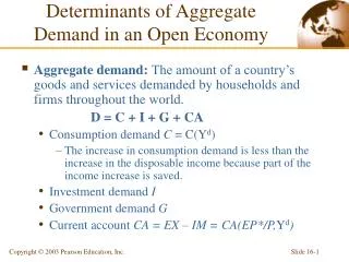
Determinants of Aggregate Demand in an Open Economy. Aggregate demand: The amount of a country’s goods and services demanded by households and firms throughout the world. D = C + I + G + CA Consumption demand C = C(Y d )

E N D
Determinants of Aggregate Demand in an Open Economy • Aggregate demand: The amount of a country’s goods and services demanded by households and firms throughout the world. D = C + I + G + CA • Consumption demand C = C(Yd) • The increase in consumption demand is less than the increase in the disposable income because part of the income increase is saved. • Investment demand I • Government demand G • Current account CA = EX – IM = CA(EP*/P,Yd)
Determinants of Aggregate Demand in an Open Economy • Real Exchange Rate q = EP*/P • Increase in q real depreciation increase in EX • Each unit of domestic output purchases fewer units of foreign output foreigners get a better deal on our output foreigners buy more of our exports volume of EX up • Increase in q can raise or lowerIM and has an ambiguous effect on CA. Volume effect: we buy fewer imports when q increases Value effect: we pay more in real terms (in units of domestic product) for the imports we do buy when q increases We assume that the volume effect of a real exchange rate change outweighs the value effect: q up CA “improves”.
Determinants of Aggregate Demand in an Open Economy Factors Determining the Current Account
Aggregate demand, D Aggregate demand function, D(EP*/P, Y – T, I, G) 45° Output (real income), Y The Equation of Aggregate Demand Aggregate Demand as a Function of Output
Aggregate demand, D Aggregate demand = aggregate output, D = Y Aggregate demand 3 1 D1 2 45° Y2 Y1 Output, Y Y3 Output market equilibrium in the short-run: The Keynesian Cross. Real output, Y, equals aggregate demand for domestic output:Y = D(EP*/P, Y – T, I, G)
Output Market Equilibrium in the Short Run: The DD Schedule Output, the Exchange Rate, and Output Market Equilibrium • With P and P* fixed, depreciation makes foreign goods and services more expensive relative to domestic goods and services. • q up (real depreciation) upward shift in aggregate demand (D) expansion of output (Y). • q down downward shift in D Y down
Aggregate demand, D D = Y Currency depreciates Aggregate demand (E2) 2 Aggregate demand (E1) 1 45° Y1 Output, Y Y2 Output Market Equilibrium in the Short Run: The DD Schedule Output Effect of a Currency Depreciation with Fixed Output Prices
Aggregate demand, D D = Y Aggregate demand (E2) Aggregate demand (E1) Y1 Y2 Output, Y Exchange rate, E DD E2 2 E1 1 Output, Y Y1 Y2 The DD Schedule: combinations of output and the exchange rate where output market is in short-run equilibrium (Y = D). DD slopes upward -- a rise in the exchange rate (depreciation) Y increases.
Output Market Equilibrium in the Short Run: The DD Schedule • Factors that Shift the DD Schedule. Increases in • Government purchases expansion DD shifts out • Taxes contraction DD shifts in • Investment expansion DD shifts out • Domestic price levels contraction in CA DD shifts in • Foreign price levels expansion in CA DD shifts out • Domestic consumption expansion DD shifts out • Demand shift between foreign and domestic goods • A disturbance that raises (lowers) aggregate demand for domestic output shifts the DD schedule to the right (left).
Aggregate demand, D D = Y Government spending rises D(E0P*/P, Y – T, I, G2) D(E0P*/P, Y – T, I, G1) Y1 Y2 Output, Y Exchange rate, E DD1 DD2 1 2 E0 Output, Y Y1 Y2 Output Market Equilibrium in the Short Run: The DD Schedule Government Demand and the Position of the DD Schedule Aggregate demand curves
AA Schedule: combinations of exchange rate and output that are consistent with asset market equilibrium (the domestic money market and the foreign exchange market). Foreign exchange market equilibrium (interest rate parity): R = R* + (Ee – E)/E where: Ee is the expected future exchange rate R is the interest rate on domestic currency deposits R* is the interest rate on foreign currency deposits Money Market equilibrium Ms/P = L(R, Y)
Exchange Rate, E Foreign exchange market 2' E2 Domestic interest rate, R 0 R2 MS P Money market Output rises Real money supply 1 Real domestic money holdings Asset Market Equilibrium in the Short Run: The AA Schedule Output and the Exchange Rate in Asset Market Equilibrium: Y up Ld up R up E down (currency appreciates) 1' E1 Domestic-currency return on foreign- currency deposits R1 L(R, Y1) L(R, Y2) 2
Exchange Rate, E 1 E1 2 E2 AA Y1 Output, Y Y2 Asset Market Equilibrium in the Short Run: The AA Schedule The AA Schedule: Y up E down (currency appreciation)
Asset Market Equilibrium in the Short Run: The AA Schedule Factors that Shift the AA Schedule • For given Y Domestic money supply: Ms up R down E up Domestic price level: P up Ms/P down R up E down Expected future exchange rate: Ee up E up Foreign interest rate: R* up E up (depreciation) Real money demand: Ld up R up E down (appreciation)
Exchange Rate, E DD 1 E1 AA Y1 Output, Y Short-Run Equilibrium for an Open Economy: Putting the DD and AA Schedules Together Short-Run Equilibrium: The Intersection of DD and AA
Exchange Rate, E DD E2 2 E3 3 1 E1 AA Y1 Output, Y Short-Run Equilibrium for an Open Economy: Putting the DD and AA Schedules Together How the Economy Reaches Its Short-Run Equilibrium: asset markets clear instantly always on AA curve $ cheap at 2 Expected $ appreciation rush to US assets $ appreciation NOW
Temporary Changes in Monetary and Fiscal Policy • Two types of government policy: • Monetary policy: works through changes in money supply. • Fiscal policy: works through changes in government spending (G) or taxes (T). • Temporary policy shifts are those that the public expects to be reversed in the near future and do not affect the long-run expected exchange rate. • Also, assume policy shifts do not influence the foreign interest rate and the foreign price level.
Exchange Rate, E DD 2 E2 1 E1 AA2 AA1 Y1 Y2 Output, Y Temporary Change in Monetary Policy Temporary Increase in the Money Supply: R down E up (depreciation) at each value of Y AA shifts up
Exchange Rate, E DD1 DD2 1 E1 2 E2 AA Y1 Output, Y Y2 Temporary Change in Fiscal Policy Temporary Fiscal Expansion: G up Y increases at each value of E DD shifts outward
Exchange Rate, E DD2 DD1 E3 3 2 E2 AA2 1 E1 AA1 Y2 Output, Y Yf Temporary Changes in Monetary and Fiscal Policy Maintaining Full Employment After a Temporary Fall in World Demand for Domestic Products: Prop up demand with fiscal or monetary stimulus (M up AA shifts up; G up DD shifts out)
Exchange Rate, E DD1 DD2 E1 1 2 E2 AA1 3 E3 AA2 Y2 Output, Y Yf Temporary Changes in Monetary and Fiscal Policy Policies to Maintain Full Employment After Money-Demand Up (Money “shortage” recession). So Increase G or Ms
Problems of Policy Formulation • Inflation bias • High inflation with no average gain in output that results from governments’ policies to prevent recession • Identifying the sources of economic changes • Identifying the durations of economic changes • The impact of fiscal policy on the government budget • Time lags in implementing policies • Policy impacts on current account balance
Permanent Shifts in Monetary and Fiscal Policy • A permanent policy shift affects not only the current value of the government’s policy instrument but also the long-run exchange rate. • This affects expectations about future exchange rates. • A Permanent Increase in the Money Supply • expected future exchange rate (Ee)rises proportionally upward shift in AA schedule is greater than that caused by an equal, but transitory, increase • need expected appreciation in the future to offset lower interest rate, R • OVERSHOOTING
Exchange Rate, E DD1 2 E2 3 1 E1 AA2 AA1 Yf Y2 Output, Y Permanent Shifts in Monetary and Fiscal Policy Short-Run Effects of a Permanent Increase in the Money Supply (E3 is newly expected long-run exchange rate)
Exchange Rate, E DD2 DD1 2 E2 3 E3 1 AA2 E1 AA3 AA1 Yf Output, Y Y2 Permanent Shifts in Monetary and Fiscal Policy Long-Run Adjustment to a Permanent Increase in Money Supply (As P rises, CA worsens (DD in) and R rises (AA down)
Exchange Rate, E DD1 DD2 E1 1 3 AA1 2 E2 AA2 Output, Y Yf Permanent Fiscal Expansion • Expected Appreciation Shifts AA Down Immediately • No Change in Output, Even in Short-Run • Complete Crowding Out
Macroeconomic Policies and the Current Account • XX schedule shows combinations of the exchange rate and output at which the CA balance stays at some desired level. • XX slopes upward: Y up Im up CA worsens unless currency depreciates. • E must increase to keep CA where it was when Y up. • XX is flatter than DD: • When currency depreciates (E up), CA improves along DD – that’s why Y increases when currency depreciates. • To keep CA from changing, E need only increase enough to offset increased imports attributable to output expansion.
Exchange Rate, E DD 2 1 E1 3 4 AA Yf Output, Y Monetary Expansion AA shifts up Depreciation CA “improves” (Point 2)Fiscal Expansion DD shifts out Appreciation CA “worsens” (Point 3 for temporary fiscal expansion; Point 4 for permanent fiscal expansion). XX
Gradual Trade Flow Adjustment and Current Account Dynamics • The J-Curve: if imports and exports adjust gradually to real exchange rate changes, the CA may follow a J-curve pattern after a real currency depreciation, first worsening and then improving. • Currency depreciation may have a contractionary initial effect on output • exchange rate overshooting will be amplified. • The J-Curve describes the time lag with which a real currency depreciation improves the CA.
Current account (in domestic output units) Long-run effect of real depreciation on the current account 3 1 2 Time Real depreciation takes place and J-curve begins End of J-curve Gradual Trade Flow Adjustment and Current Account Dynamics The J-Curve
Gradual Trade Flow Adjustment and Current Account Dynamics • Exchange Rate Pass-Through and Inflation • The CA in the DD-AA model has assumed that nominal exchange rate changes cause proportional changes in the real exchange rates in the short run. • Degree of Pass-through • It is the percentage by which import prices rise when the home currency depreciates by 1%. • In the DD-AA model, the degree of pass-through is 1. • Exchange rate pass-through can be incomplete because of international market segmentation. • Currency movements have less-than-proportional effects on the relative prices determining trade volumes.
Summary • The aggregate demand for an open economy’s output consists of four components: consumption demand, investment demand, government demand, and the current account. • Output is determined in the short run by the equality of aggregate demand and aggregate supply. • The economy’s short-run equilibrium occurs at the exchange rate and output level.
Summary • A temporary increase in the money supply causes a depreciation of the currency and a rise in output. • Permanent shifts in the money supply cause sharper exchange rate movements and therefore have stronger short-run effects on output than transitory shifts. • If exports and imports adjust gradually to real exchange rate changes, the current account may follow a J-curve pattern after a real currency depreciation, first worsening and then improving.
Interest rate, R LM 1 R1 IS Y1 Output, Y Appendix I: The IS-LM Model and the DD-AA Model Figure 16AI-1: Short-Run Equilibrium in the IS-LM Model
Interest rate, R LM1 LM2 1 1´ R1 2 R2 2´ 3 R3 3´ IS2 IS1 E2 E3 E1 Y1 Y2 Y3 Output, Y Appendix I: The IS-LM Model and the DD-AA Model Figure 16AI-2: Effects of Permanent and Temporary Increases in the Money Supply in the IS-LM Model Expected domestic-currency return on foreign-currency deposits Exchange rate, E ( increasing)
Interest rate, R LM 2´ R2 2 1 3´ 1´ R1 IS2 IS1 E1 E2 E3 Y2 Yf Output, Y Appendix I: The IS-LM Model and the DD-AA Model Figure 16AI-3: Effects of Permanent and Temporary Fiscal Expansions in the IS-LM Model Expected domestic-currency return on foreign-currency deposits Exchange rate, E ( increasing)
Appendix II: Intertemporal Trade and Consumption Demand Future consumption Intertemporal budget constraints Intertemporal budget constraints 2 D2F 1 D1F = Q1F 2´ Indifference curves Present consumption D1P = Q1P Q2P D2P Figure 16AII-1: Change in Output and Saving
Appendix III: The Marshall-Lerner Condition and Empirical Estimates of Trade Elasticities Table 16AIII-1: Estimated Price Elasticities for International Trade in Manufactured Goods