Aggregate Demand
Aggregate Demand. AGGREGATE DEMAND, AGGREGATE SUPPLY, AND MODERN MACROECONOMICS Part 1. Laugher Curve. We adults do have something in common with today’s teenagers. They listen to rock groups and we listen to economists. None of us understands a word they’re saying. Jean Stapleton.

Aggregate Demand
E N D
Presentation Transcript
Aggregate Demand AGGREGATE DEMAND, AGGREGATE SUPPLY, AND MODERN MACROECONOMICS Part 1
Laugher Curve We adults do have something in common with today’s teenagers. They listen to rock groups and we listen to economists. None of us understands a word they’re saying. Jean Stapleton
The AS/AD Model • The AS/AD model consists of three curves: • The short-run aggregate supply curve. • The aggregate demand curve. • The long-run aggregate supply curve.
The AS/AD Model • The AS/AD model is fundamentally different from the microeconomic supply/demand model.
The AS/AD Model • Microeconomic supply/demand curves concern the price and quantity of a single good. • Price is measured on the vertical axis and quantity is measured on the horizontal axis. • The shapes are based on the concepts of substitution and opportunity cost.
The AS/AD Model • In the AS/AD model the price of everything is on the vertical axis and aggregate output is on the horizontal axis.
The AS/AD Model • The AS/AD model is an historical model that starts at a point in time and says what will happen when changes affect the economy.
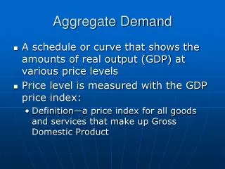
The Aggregate Demand Curve • The aggregate demand (AD) curve shows how a change in the price level changes aggregate expenditures on all goods and services in an economy. • It shows the level of expenditures that would take place at every price level in the economy.
The Slope of the AD Curve • The AD is a downward sloping curve. • Aggregate demand is composed of the sum of aggregate expenditures. Expenditures = C + I + G +(X - M)
The Slope of the AD Curve • The slope of the AD curve is determined by the wealth effect, the interest rate effect, the international effect, and the multiplier effect.
The Wealth Effect • Wealth effect – a fall in the price level will make the holders of money and other financial assets richer, so they buy more. • Most economists accept the logic of the wealth effect, however, they do not see the effect as strong.
The Interest Rate Effect • Interest rate effect – the effect a lower price level has on investment expenditures through the effect that a change in the price level has on interest rates.
The Interest Rate Effect • The interest rate effect works as follows: a decrease in the price level increase of real cash banks have more money to lend interest rates fall investment expenditures increase
The International Effect • Internationaleffect – as the price level falls (assuming exchange rates do not change), net exports will rise.
The International Effect • The international effect works as follows: a decrease in the price level in the U.S. the fall in price of U.S. goods relative to foreign goods U.S. goods become more competitive internationally U.S. exports rise and U.S. imports fall
The Multiplier Effect • Initial changes in expenditures set in motion a process in the economy that amplifies the initial effects. • Multiplier effect – the amplification of initial changes in expenditures.
The Multiplier Effect • The multiplier effect works as follows: an increase in the price level in the U.S. U.S. exports fall and U.S. imports rise U.S. firms lose sales and cut output U.S. incomes fall U.S. households buy less U.S. firms cut back again and so on
The Multiplier Effect • The multiplier effect amplifies the initial wealth, interest rate, and international effects, making the AD curve flatter than it would have been.
Multiplier effect The AD Curve is Downward Sloping for 4 Reasons 1. Wealth Effect P value of money so that people feel wealthier spending Price level Wealth, interest rate, and international effects 2. Interest Rate Effect P real money supply and supply of loans interest rates investment P0 3. International Effect P of U.S. goods exports and imports P1 AD 4. Multiplier Effect Amplifies the wealth, interest rate, and international effects so that the AD is flatter Y0 Y1 Ye Real output
How Steep Is the AD Curve • Most economists agree that small changes in the price level result in relatively small changes in expenditures. • This gives the AD curve a very steep slope.
The AD Curve Shifts for 5 Reasons 1. Foreign Income • Foreign income exports AD • 2. Exchange Rates Depreciation of the $ exports AD • 3. Expectations Optimism and expectations of future prices AD
The AD Curve Shifts for 5 Reasons 4. Distribution of Income Wage portion of income AD • 5. Government AD management policies • Fiscal policy Tax and/or government spending AD • Monetary policy Federal Reserve money supply interest rates spending AD • Multiplier Effects Magnify the initial shift of AD
200 100 AD1 Shifts in the AD Curve Initial effect = 100 increase in exports Price level Multiplier effect = 200 Change in total expenditures = 300 P0 AD0 Real output