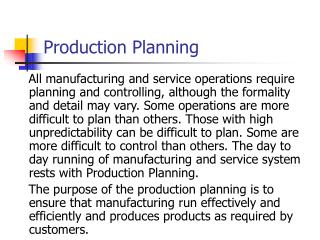
Dynamic Inventory and Workforce Scheduling for Singapore Electric Generator Production
This model analyzes the production and inventory dynamics of the Singapore Electric Generator, focusing on unit costs and inventory management over several months. It incorporates workforce scheduling to meet delivery requirements while minimizing costs. The inventory and production limits are taken into account, ensuring that the constraints are met efficiently. A solver model is formulated to minimize excess worker requirements while maintaining adequate staffing levels to meet demand across the week. This comprehensive approach addresses the complexities of production planning and workforce management.

Dynamic Inventory and Workforce Scheduling for Singapore Electric Generator Production
E N D
Presentation Transcript
Production Planning Basic Inventory Model Workforce Scheduling Enhance Modeling Skills Dynamic Models
Dynamic Inventory Model • Modeling Time • Modeling Inventory • Unusual Network Example
Singapore Electric Generator • Singapore Electric Generator Production • Unit Costs Jan Feb Mar Apr. May Production $ 28.00 $ 27.00 $ 27.80 $ 29.00 • Inventory $ 0.30 $ 0.30 $ 0.30 $ 0.30 • Production Qty 0 0 0 0 • Production Limits 60 62 64 66 • Beginning Inventory 15 -43 -79 -113 • Delivery Reqmts 58 36 34 59 Minimum • Ending Inventory (43) (79) (113) (172) 7 • Production Cost $ -$ -$ -$ - • Inventory Cost $ (4.20) $ (18.30) $ (28.80) $ (42.75) Total • Total Cost $ (4.20) $ (18.30) $ (28.80) $ (42.75) $ (94.05)
Inventory • Balancing Your Checkbook • Previous Balance + Income -Expenses = New Balance • Modeling Dynamic Inventory • Starting Inv. + Production -Shipments = Ending Inv.
Average Balances • Assuming Smooth Cash Flows Averages (Starting + Ending)/2
Challenge • Formulate a Solver Model
Singapore Electric Generator • Singapore Electric Generator Production • Unit Costs Jan Feb Mar Apr. May Production $ 28.00 $ 27.00 $ 27.80 $ 29.00 • Inventory $ 0.30 $ 0.30 $ 0.30 $ 0.30 • Production Qty 0 0 0 0 • Production Limits 60 62 64 66 • Beginning Inventory 15 -43 -79 -113 • Delivery Reqmts 58 36 34 59 Minimum • Ending Inventory (43) (79) (113) (172) 7 • Production Cost $ -$ -$ -$ - • Inventory Cost $ (4.20) $ (18.30) $ (28.80) $ (42.75) Total • Total Cost $ (4.20) $ (18.30) $ (28.80) $ (42.75) $ (94.05)
A Network Formulation Jan. mfg. Feb. mfg. Mar. mfg. Apr. mfg. Supply ≤ Prod. Limits Production Variables Dec. Inv. Jan. Inv. Mar. Inv. May Inv. Feb. Inv. Apr. Inv. Shipment Quantities Inventory Variables Feb. dem. Mar. dem. Apr. dem. Jan. dem. Demand ≥ req
A Network Formulation Singapore Electric Generator Production Unit Costs Dec Jan Feb Mar Apr. May Production $ 28.00 $ 27.00 $ 27.80 $ 29.00 Inventory $ 0.30 $ 0.30 $ 0.30 $ 0.30 Production Qty 0 0 0 0 Production Limits 60 62 64 66 Delivery Reqmts 58 36 34 59 Calc. Ending Inv. -43 (36) (34) (59) Minimum Ending Inventory 15 - - - - 7 Production Cost $ - $ - $ - $ - Inventory Cost $ 2.25 $ - $ - $ - Total Total Cost $ 2.25 $ - $ - $ - $ 2.25
Another View s.t. InitialBalance: Production['Jan'] -EndingInv['Jan'] = 43 s.t. MonthlyBalances['Feb']: Production['Feb'] + EndingInv['Jan'] -EndingInv['Feb'] = 36 s.t. MonthlyBalances['Mar']: Production['Mar'] + EndingInv['Feb'] -EndingInv['Mar'] = 34 s.t. MonthlyBalances['Apr']: Production['Apr'] + EndingInv['Mar'] -EndingInv['Apr'] = 59 s.t. FinalBalance: EndingInv['Apr'] >= 7
Scheduling Postal Workers • Each postal worker works for 5 consecutive days, • followed by 2 days off, repeated weekly. Day Mon Tues Wed Thurs Fri Sat Sun Demand 17 13 15 19 14 16 11 • Minimize the number of postal workers (FTE’s)
Challenge • Formulate a Solver Model
Formulating the LP Scheduling Postal Workers • Shift Mon - Tues - Wed - Thurs - Fri - Sat - Sun – • Fri Sat Sun Mon Tues Wed Thurs • Day Demand • Mon 1 1 1 1 1 17 • Tues 1 1 1 1 1 13 • Wed 1 1 1 1 1 15 • Thurs 1 1 1 1 1 19 • Fri 1 1 1 1 1 14 • Sat 1 1 1 1 1 16 • Sun 1 1 1 1 1 11
Formulating as an LP • The Objective • Total Workers Required • Minimize $I$5 • The decision variables • The number of workers assigned to each shift • $B$5:$H$5 • The Constraints • Enough workers each day • $I$6:$I$12 >= $J$6:$J$12
The linear program • Minimize z = MF + TS + WSu+ ThM+ FT + SW + SuTh • subject to MF + ThM+ FT + SW + SuTh ≥ 17 MF + TS + FT + SW + SuTh ≥ 13 MF + TS + WSu+ SW + SuTh ≥ 15 MF + TS + WSu+ ThM+ SuTh ≥ 19 MF + TS + WSu + ThM + FT ≥ 14 TS + WSu + ThM + FT + SW ≥ 16 WSu + ThM+ FT + SW + SuTh ≥ 11 Non-negativity
The Decision Variable Decision • Would it be possible to have the variables be the number of workers on each day? • Conclusion: sometimes the decision variables • incorporate constraints of the problem. • Hard to do this well, but worth keeping in mind • We will see more of this in integer programming.
Enhancement • Some days we will have too many workers • Excess • Only concerned with the largest excess • Minimize the largest Excess
Challenge • Formulate a Solver Model
Formulating the LP Scheduling Postal Workers • Shift Mon - Tues - Wed - Thurs - Fri - Sat - Sun – • Fri Sat Sun Mon Tues Wed Thurs • Day Demand • Mon 1 1 1 1 1 17 • Tues 1 1 1 1 1 13 • Wed 1 1 1 1 1 15 • Thurs 1 1 1 1 1 19 • Fri 1 1 1 1 1 14 • Sat 1 1 1 1 1 16 • Sun 1 1 1 1 1 11
Minimize the Maximum • Min Max{XS[Mon], XS[Tues], …} • Min Z • S.t. Z ≥ XS[Mon] • S.t. Z ≥ XS[Tues] • … • S.t. MF + ThM + FT + SW + SuTh– XS[Mon] = 17 • S.t. MF + TS + FT + SW + SuTh– XS[Tues] = 13 • ….
Enhancement • Ensure at least 30% of the workers have Sunday off • Formulate a Solver Model
Formulating the LP Scheduling Postal Workers • Shift Mon - Tues - Wed - Thurs - Fri - Sat - Sun – • Fri Sat Sun Mon Tues Wed Thurs • Day Demand • Mon 1 1 1 1 1 17 • Tues 1 1 1 1 1 13 • Wed 1 1 1 1 1 15 • Thurs 1 1 1 1 1 19 • Fri 1 1 1 1 1 14 • Sat 1 1 1 1 1 16 • Sun 1 1 1 1 1 11
The linear program • Minimize z = MF + TS + WSu+ ThM+ FT + SW + SuTh • subject to MF + ThM+ FT + SW + SuTh ≥ 17 MF + TS + FT + SW + SuTh ≥ 13 MF + TS + WSu+ SW + SuTh ≥ 15 MF + TS + WSu+ ThM+ SuTh ≥ 19 MF + TS + WSu + ThM + FT ≥ 14 TS + WSu + ThM + FT + SW ≥ 16 WSu + ThM+ FT + SW + SuTh ≥ 11 .7(MF + TS) -0.3*(WSu + ThM + FT + SW + SuTh) ≥ 0 Non-negativity
Summary • More LP Modeling • LPs are more general than Networks • Modeling Time • Clever choices of decision variables