Understanding Random Variables and Probability Distributions in Statistics
This chapter delves into the concepts of random variables, highlighting both discrete and continuous types. Readers will learn how to define a random variable, explore its probability mass function (pmf) and probability density function (pdf), and calculate expectations, variance, and standard deviation. Practical examples, such as rolling dice and traffic accidents, illustrate how randomness influences real-world phenomena. The chapter emphasizes the importance of these concepts in predicting and controlling outcomes in uncertain situations, essential for students and professionals in statistics and data analysis.


Understanding Random Variables and Probability Distributions in Statistics
E N D
Presentation Transcript
Chapter 2: Random Variable and Probability Distributions zlyang@smu.edu.sg http://www.mysmu.edu/faculty/zlyang/ Yang Zhenlin
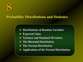
Chapter Contents • Random Variable (r.v.) • Discrete r.v. • Continuous r.v. • Distribution of a Random Variable • Probability mass function (pmf) • Probability density function (pdf) • Expectation of a Random Variable • Variance and Standard Deviation • Moment Generating Function
Random Variable In real-world problems, we are often faced with one or more quantities that do not have fixed values. The values of such quantities depend on random actions and they change from one experiment to another, Number of babies born in a certain hospital Number of traffic accidents occurred on a road per month The amount of rainfall in Singapore per year The starting price of a stock each day, etc. In probability, quantities introduced in these diverse examples are called Random Variables. Study the properties of random variables allows us to have a better understanding on the real-world phenomena, and to control or to predict their behavior, … .
Random Variable where, for example, p2 = P(X=2) = P{(1,1)} = 1/36, p3 = P(X=3) = P{(1,2), (2,1)} = 2/36, p7 = P(X=7) = P{(1,6), (6,1), (2,5), (5,2), (3,4), (4,3)} = 6/36 Example 2.1 If in the experiment of rolling two fair dice, X is the sum, then X is a variable. Since the value of X changes from one experiment to another, X is also a "random variable". The possible values of X and the corresponding probabilities are summarized as follows:
Random Variable Definition 2.1. Let S be the sample space of an experiment. A real-valued function X defined on S and taking values in R (the set of real numbers) is called a random variable (r.v.) if for each interval IR, the inverse image {e: X(e) I } is an event. • In Example 2.1, numerical values of X depend on the outcomes of the experiment, e.g., • if the outcome e = (2,3), then X = 2+3 = 5, • if e = (5,6), then X = 5+6 = 11, etc. Thus, X is a real-valued function. • On the other hand, if, for example, X = 3, then it must be that e = (1,2) or (2,1). Therefore, the inverse image of the function X is an event!
Random Variable All probabilities add up to 1: Example 2.2 Suppose that we toss a coin having a probability p of coming up heads, until the first head appears. Let N denote the number of flips required, then assuming the outcome of successive flips are independent, N is a random variable taking values 1, 2, 3, …, with respective probabilities P{N =1} = P(H) = p, P{N =2} = P(TH) = (1p)p, P{N =3} = P(TTH) = (1p)2p,
Distribution of a Random Variable Definition 2.2 (Cumulative Distribution Function) The cumulative distribution function (CDF) of a random variable X is defined by, F(x) = P{X ≤ x}, for any real x. A function F(x) is a CDF if and only if it satisfies: (a) limx F(x) = 0 and limx F(x) = 1 (b) limh0F(x+h)= F(x), h > 0 (right continuous) (c) a < b implies F(a) ≤ F(b) (nondecreasing). F(x) “cumulates” all of the probabilities of the values of X up to and including x.
Distribution of a Random Variable Example 2.3. A four-sided die has a different number, 1, 2, 3, or 4, affixed to each side. On each roll, each of the four numbers is equally likely to occur. A game consists of rolling the die twice. If X represents the maximum of the two rolls, then X is a random variable. Find and sketch the CDF of X Solution: Possible values for X are 1, 2, 3, and 4, and the corresponding probabilities are: P(X = 1) = P{(1,1)} = 1/16 P(X = 2) = P{(1,2), (2,1), (2,2)} = 3/16 P(X = 3) = P{(1,3), (2,3), (3, 3), (3,2), (3,1)} = 5/16 P(X = 4) = P{(1,4), (2,4), (3,4), (4,4), (4,3), (4,2), (4,1)} = 7/16. Thus, the CDF of X is,
Distribution of a Random Variable Example 2.4. A function is specified as follows. F(x) = • Verify that it is a CDF. • Plot F(x) and calculate: P(X < 2), P(X = 2), and • P(1 ≤ X < 3). Solution: (a) … , (b) : P(X < 2) = F(2–) = 1/2. P(X = 2) = F(2) – F(2–) = (2/12+1/2)–1/2 = 1/6. P(1 ≤ X < 3) = P(X < 3) – P(X < 1) = F(3–) – F(1–) = (3/12+1/2) – 1/4 = 1/2.
Distribution of a Random Variable Definition 2.3 (Discrete R.V. and Probability Mass Function)If the set of all possible values of a random variable, X, is a countable set, x1, x2, . . . , xn, or x1, x2, . . ., then X is called a discrete random variable. The function p(x) = P(X = x), x = x1, x2, . . . that assigns the probability to each possible value of X will be called probability mass function (pmf). So, pmf tells how the probabilities are distributed across the values of r.v. X. Note. Random variables can be classified as discrete, continuous, or mixed. The function given in Example 2.4 is a mixed CDF which has “jumps” at certain points. We will concentrate on pure discrete and pure continuous types of random variables.
Distribution of a Random Variable A function p(x) is a pmf if and only if (i) p(x) ≥ 0 for all x, and (ii) Example 2.5. Is each of the following functions a pmf? If it is, find the constant k. (a) p(x) = k(1/2)x, x = 0, 1, 2, . . . (b) p(x) = k [(1/2)x – 1/2], x = –2, –1, 0, 1, 2. Solution: (a) p(x) > 0 for all x = 0, 1, 2, . . . ; and (b) Since p(0) = k/2, and p(2) = –k/4, the two values of the function have opposite signs no matter what value k takes. Therefore, it is impossible for p(x) to be always nonnegative, and hence p(x) cannot be a pmf.
Distribution of a Random Variable Definition 2.4 (Continuous R.V. and Probability Density Function)A r.v. X is said to be a continuous random variable if there exists a nonnegative function f, defined for all real x (– , ), such that for any set B of real numbers P{X B} = . The function f is called the probability density function (pdf) of the r.v. X. So, pdff(x) tells how likely values of r.v. X occurs around x. The r.v's introduced above take countable number of values. However, many social phenomena can only be described by variables with uncountable values, e.g., arrival time of a train, lifetime of a transistor, etc.
Distribution of a Random Variable Example 2.6 A CDF has the following expression F(x) = Sketch the graph of F(x) and find the pdf f(x). Solution: The graph of F(x) is shown below. Clearly, F(x) is not differentiable at x = 0, 0.5 and 1.5. Take the ‘right’ derivatives, i.e., f(0) = 1, f(0.5) = 0.5, and f(1.5) = 0, we then have
Distribution of a Random Variable A function f(x) is a pdf if and only if it satisfies the properties (i)f(x) ≥ 0 for all x and (ii) Example 2.7 A machine produces copper wire, and occasionally there is a flaw at some point along the wire. The length of the wire (in meters) produced between successive flaws is a continuous r.v. X with pdf of the form: f(x) = c(1+x)3, x > 0, where c is a constant. Find c, and CDF.
Expectation of a Random Variable Definition 2.5. (Expectation)The expected value of a discrete r.v. X with pmf p(x) is defined by = E(X) = i.e., a weighted average of all possible values of X. It is also called mean of the population represented by X. Expected value of a discrete r.v. is just the weighted average of the possible values of X, weighted by their chances to occur. The expected value of a continuous r.v. with pdf f(x) is defined by = E(X) = if the integral is absolutely convergent. Otherwise we say that E(X) does not exist.
Expectation of a Random Variable Expectation is an extremely important concept in summarizing characteristics of distributions. It gives a measure of central tendency. It has following simple but important property: • If a and b are constants, then • E[aX + b] = a E[X] + b In Example 2.1, X is the sum of the two numbers shown on the two dice. The expected sum is: E(X) =
Function of a Random Variable • The following results are important: • If X is a r.v., then a function of it, u(X), is also a r.v. , • E[u(X) ] = , if X is a discrete r.v. with pmf p(x), • E[u(X) ] = , if X is a continuous r.v. with pdf f(x). Example 2.8 The r.v. X has pmf p(x) = 1/3, for x = 1, 0, 1. Find E(X) and E(X2). Solution: The above result says that the expectation of the r.v., u(X), can simply be found through the distribution of the original r.v. X !
Variance of a Random Variable Another important quantity of interest is the variance of a r.v. X, denoted by Var(X), which is defined by Var(X) = E[(X –)2], where = E(X). A related quantity is the standard deviation, (X) = {Var(X)}1/2. • Variance and standard deviation (sd) measure how much the values of X vary around its mean . As (X –)2 is a function of X, i.e., u(X) = (X –)2, from the results given in the last slide, we have Var(X) = , if X is discrete with pmf p(x), Var(X) = , if X is continuous with pdf f(x).
Variance of a Random Variable We note in Example 2.9 Var(X) and Var(Y) are the same. Why? • If X is a r.v. with mean , and a and b are arbitrary constants, then • E(aX + b) = aE(X) + b • Var(X) = E(X2) – 2 • Var(aX + b) = a2Var(X) • (aX + b) = |a|(X). To show third result, Var(aX + b) = E[(aX + b – E[aX + b])2] = E[(aX + b – aE[X ] – b)2] = E[(aX –aE[X ])2] = E[a 2(X –E[X ])2] = a 2E[(X –E[X ])2] = a2Var(X) To show the second result, Var(X) = E[(X –)2] = E(X2 –2X+ 2) = E(X2) –2 E(X)+ 2 = E(X2) – 2
Variance of a Random Variable Example 2.10. The monthly sales at a computer store have a mean of $25,000 and a standard deviation of $4,000. Profits are 30% of the sales less fixed costs of $6,000. Find the mean and standard deviation of the monthly profit. Solution:Let X = Sales. E(X) = 25,000, and Var(X) = 4,0002 Let Y = Profit. Then, Y = .30(X) – 6,000. E(Profit) = E(Y) = .30 E(X) – 6,000 = (.30)(25,000) – 6,000 = 1,500. Var(Profit) = Var(Y) = Var[(.30)(X) – 6,000] = (.30)2Var(X) = 1,440,000 (Profit) = (Y) = 0.3(X) = 1,200.
Moment Generating Function • The mean, variance and standard deviation are important characteristics of a distribution. • For some distributions, it is rather difficult to compute these quantities directly. • A special function defined below can help. More importantly, the uniqueness property of this function often help to find the distribution of some useful functions of r.v.s. Definition 2.12 (Moment-Generating Function)Let X be a random variable, discrete or continuous. If there exists a positive number h such that M(t) = E(etX) exists and is finite for –h < t < h, then M(t) is called the Moment-Generating Function (MGF) of X.
Moment Generating Function • Why is it called the Moment Generating Function? • because it generates moments. • What are the moments? • the term ‘moment’ is from mechanics, representing the product of a distance and its weight. • So, xi p(xi) is a moment, and xi p(xi) or E(X) is the moment of the ‘system’. • In statistics, E(X), E(X2), E(X3), …, are the 1st, 2nd , 3rd, …, moments about the origin; • E(X), E[(X)2], E[(X)3], etc, are the 1st, 2nd , 3rdcentral moments, or moments about the mean. • See p67 of text for details.
Moment Generating Function • Property of MGF: • M.G.F., if it exists, completely determines the distribution function. In other words, if two random variables, assuming the same set of values, have the same M.G.F., they must have the same distribution function. • E(Xr) = M(r)(0), the rth derivative of M(t) evaluated at 0. We use a discrete r.v.s to demonstrate these properties: if X and Y have possible values {v1, v2, …}, and pmfs p(x) and q(x), then, Thus, if MX(t) = MY(t), it must be that p(vi) = q(vi), i = 1, 2, …
Moment Generating Function To understand the property E(Xr) = M(r)(0), we have Thus, Thus, In general,
Moment Generating Function Example 2.11. If X has the MGF, then, as the coefficients of the e terms are probabilities, the probabilities must be 3/6, 2/6, and 1/6; the values beside t are the values of X, which are 1, 2, and 3. The pmf of X is Example 2.12. Suppose the MGF of X is Find the distribution of X.
Moment Generating Function Solution: Until we expand M(t), we cannot detect the coefficients of Recall: we have, That is, P(X = x) = (1/2)x, for positive integer x; the pmf of X is thus,