Understanding Probability in Random Behavior Modeling
This overview details how statisticians utilize probability to model uncertainty in events. It illustrates key concepts such as defining events, sample spaces, and conditional probabilities, highlighting their application in real-world scenarios, like evaluating product reliability. The estimation of probabilities, both objective and subjective, and the impact of assumptions on these probabilities are explored. Examples from manufacturing contexts, particularly related to product quality and order fulfillment likelihoods, illustrate these principles, emphasizing the importance of accurate probability assessment.

Understanding Probability in Random Behavior Modeling
E N D
Presentation Transcript
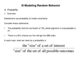
III Modeling Random Behavior • Probability • Overview • Statisticians use probability to model uncertainty. • Consider-these statements: • The probability that the next batch of Ti02 (white pigment) is unacceptable is .01. • There is a 25% chance our firm will get the IBM order. • In each case, what we mean by a probability is
Some notation will aid our discussion. • An event is a set of possible outcomes of interest. • The sample space, S, is the set of all possible outcomes. • If A is an event, the probability that A occurs is • Note: • 0 ≤ P(A) ≤ 1 • P(S) = 1 • Probability may be either objective (based on prior experience) or poorly subjective. • Ultimately, the accuracy of specific probabilities depends on assumptions. • If the assumptions upon which we base a specific probability are wrong, then we should not expect the specific probability to be any good.
Example: Making Nickel Battery Plate A particular process for making nickel battery plate requires an operator to sift nickel powder into a frame. The process uses a very tight weight specification, which is difficult to make. The supervisor monitored the last 1000 attempts made by an operator. The operator successfully made the specification 379 times. One way to get the probability of a successful attempt is
The supervisor noted, however, that the operator seemed to get better over time. In this case, the supervisor may believe that the actual probability is something larger than .379. A perfectly reasonable, but subjective, estimate of the probability of a successful attempt is 0.4.
2. Making Inferences Using Probabilities. Suppose the supervisor really believes that the probability of a successful attempt is 0.4. Suppose further that out of the next 50 attempts, she is never successful. Would you now believe that the probability of a success is still 0.4? OF COURSE NOT! Consider another scenario. Suppose the first attempt is unsuccessful. Do you have good reason to believe that the true probability of a success is not 0.4?
Suppose the first two attempts are unsuccessful. Suppose the first three are unsuccessful. At what point do we begin to believe that the probability really is not 0.4? The answer lies in calculating the probability of seeing y in a row assuming a probability of 0.4. Once that probability is small enough, we can reasonably conclude that the true probability is not 0.4
3. Conditional Probability Often, two events are related. Knowing the relationship between the two events allows us to model the behavior of one event in terms of the other. Conditional Probability quantifies the chances of one event occuring given that the other occurs. We denote the probability that an event A occurs given that the event B has occured by P(A|B). The key to conditional probability: the intersection of the two events defines the nature of their relationship.
This concept is best illustrated by an example: Personal Computers • A major manufacturer of personal computers has introduced a new p.c. • As with most new products, there seem to be some problems. • This manufacturer offers a one-year warranty on this model. • Let • A be the event that the hard drive on a specific computer fails within one year. • B be the event that the floppy drive on a specific computer fails within one year. • Consider a specific computer whose floppy drive has failed.
In this case, we know that the event B has occured. What now is the probability that this same computer will have its hard drive fail? What we seek is P(A|B). Note: once we know that B has occured, the sample space of interest is restricted to B. Similarly, once we know that B has occured, the set of interest is restricted to that portion of A which resides in B, A ∩ B.
Definition: Conditional Probability Let A and B be events in S. The conditional probability of B given that A has occurred is if P(A) > 0. Similarly, the conditional probability of A given that B has occurred is if P(B) > 0.
Example: Personal Computers - Continued The reliability engineers have determined that: P(A) = .02 P(B) = .05 P(A U B) = .01 Note: P(A U B) is the probability that both the hard and floppy drives on a specific computer fail within one year). The conditional probability that the hard drive fails given that the floppy drive fails is As a result, if we know that the floppy drive failed on a given machine, then the probability the hard drive will fail also is 20%.
4. Independence • In many engineering situations, two events have no real relationship. • Knowing that one event has occured offers no new information about the chances the other will occur. • We call two such events independent. • Independence is important for a number of reasons: • many engineering events either are independent or close enough for a first approximation • independence provides a powerful basis for modeling the joint behavior of several events • the formal concept of a random sample assumes that the observations are independent.
Definition: Independence Let A, B be events in S. A and B are said to be independent if P(A | B) = P(A) Similarly, if A and B are independent, then P(B | A) = P(B)
Example: Personal Computer - Continued Recall: P(A) = .02 P(B) = .05 P(A | B) = .20 Note: the hard drive failing and the floppy drive failing are not independent events because P(A | B) ≠ P(A) Why? Many personal computer designs use the floppy drive as an expensive air filter. As the floppy drive gets dirty, it increases the likelihood of it failing. Also, as the floppy get dirty, the p.c. does not vent heat as well, which increases the likelihood that the hard drive fails.
5. Basic Rules of Probability • 0 ≤ P(A) ≤ 1. • If Ø is the empty set, then P(Ø) = 0. • 3. The Probability of Complements • If A is an event in some sample space S, then the complement of the • set A relative to S is the set of outcomes in S which are not in • A. • We denote the complement of A by Ā. • P(Ā) = 1 - P(A) • 4. The Additive Law of Probability • If A and B are events in S, then the union of A and B, denoted by A U B, is the set of outcomes either in A or in B or in both.
The Additive Law of Probability is P(A U B) = P(A) + P(B) - P(A ∩ B) If A and B are mutually exclusive, then A ∩ B = Ø and P(A ∩ B) = 0; thus, P(A U B) = P(A) + P(B) 5. The Multiplicative Law of Probability If A and B are events in S, with P(A) > 0 and P(B) > 0, then Thus, P(A ∩ B) = P(A) • P(B | A) Similarly, P(A ∩ B) = P(B) • P(A | B)
If A and B are independent, then P(A | B) = P(A) P(B | A) = P(B) Thus, if A and B are independent, then P(A ∩ B) = P(A) • P(B) This property is a very powerful result, making independence quite important for finding the probabilities associated with the intersections of events.
6. Simplest Form of the Law of Total Probability • Let A and B be events in S. We may partition B into two parts: • that which overlaps A, A ∩ B, and • that which overlaps Ā, Ā ∩ B • Thus, • P(B) = P(A ∩ B) + P(Ā ∩ B) • = P(A) • P(B | A) + P(Ā) • P(B | Ā) • 7. The Simplest Form of Bayes Rule • Let A and B be events in S. • Suppose we are given P(A),P(B | A), and P(B | Ā)
Example for Toothpaste Containers A toothpaste company uses four injection molding processes to make its toothpaste containers. These are older pieces of equipment and subject to problems. Event DescriptionProb A Machine 1 has a problem on any specific day 0.1 B Machine 2 has a problem on any specific day 0.2 C Machine 3 has a problem on any specific day 0.05 D Machine 4 has a problem on any specific day 0.05 What is the probability that no problems occur on any specific day?
Note: no problems means • Machine 1 has no problems, , and • Machine 2 has no problems, , and • Machine 3 has no problems, , and • Machine 4 has no problems, • Thus, we seek the probability of an intersection. • If we can assume independence, then the probability of the intersection is the product of the individual probabilities. • P(no problems)
B. Discrete Random Variables • Overview • Let Y be the number of problems that occur on a given day. • What does Y = 0 mean? • No problems, which is • What does Y=1 mean? • Exactly one problem, which is • Note: Each one of these events is mutually exclusive of the others; thus, • P(Y = 1) • When all is said and done P(Y = 1) = 0.30305
In a similar manner, we can show that P(Y = 2) = 0.04455 P(Y = 3) = 0.00255 P(Y = 4) = 0.00005 Y is an example of a random variable. We describe the behavior of a random variable by its distribution. Every random variable has a cumulative distribution function, F(Y) defined by F(y) = P(Y ≤ y) In our case yF(y) 0 0.64980 1 0.95285 2 0.99740 3 0.99995 4 1.00000
There are two types of random variables: • Discrete, which have a countable number of possible values • Continuous, which are over a continuum (have an uncountable number of value). • Discrete random variables have a probability function, p(y) defined by • p(y) = P(Y = y) • For our example • yp(y) • 0 0.64980 • 1 0.30305 • 2 0.04455 • 3 0.00255 • 4 0.00005
Expected Values • Random variables and their distributions provide a way to model random behavior and populations. • Parameters are important characteristics of populations. • For example, • the typical number of problems which occur each day • the variability in the number of problems which occur. • We have already outlined a distribution which describes this number. • We can use this distribution to define measures of typical and of variability.
Let Y be the discrete random variable of interest. For example, let Y be the number of problems which occur on any given day with the injection molding process for toothpaste tubes. A measure of the typical value for Y is the population example, or the expected value for Y. A measure of the variability of Y is the population variance, σ2, defined by where
What are What are the units of the population variance? • As a result, we often use the population standard deviation, σ, as a measure of variability where • Many texts note that virtually all of the data for a particular distribution should fall in the interval μ ± 3σ (the empirical rule). • In general, we should take this recommendation with a grain of salt because very skewed or heavy tailed distributions are exceptions. • The empirical rule does point out that we can begin to describe the behavior of many distributions with just two measures: • the population mean and • the population standard deviation. • Many engineers commonly evaluate their data using this notion of the mean plus or minus three standard deviations.
Example: Number of problems with an injection molding process for toothpaste tube. Note: μ ± 3σ = 0.4 ± 3(0.587) = (-1.361, 2.161) The chances of seeing data within this interval are 99.74\%.
Binomial Distribution • The manufacturer of nickel battery plate has imposed a tight initial weight specification which is difficult to meet. • Consider the next three attempts made by an operator who has a 40 % chance of being successful. • Let S represent a successful attempt. • Let F represent a failed attempt. • Let Y represent the number of successful attempts she makes. • Consider the probability that exactly two out of these three attempts are successful, i.e, P(Y = 2). • The possible ways she can get exactly two successful attempts are • (SSF) (SFS) (FSS)
Since these events are mutually exclusive, then the probability of exactly two successful attempts is P(Y = 2) = P(SSF) + P(SFS) + P(FSS) In this situation, we can reasonably assume that each attempt is independent of the others. Let p be the probability that she succeeds in meeting the weight specification on any given attempt. Thus, p = 0.4. Let q = 1 - p be the probability that she fails. In this specific case, q = .6. Since each attempt is independent of the others, then P(SSF) = P(S) • P(S) • P(F) = p • p • q = p2 • q = 0.096 P(SFS) = P(S) • P(F) • P(S) = p • q • p = p2 • q = 0.096 P(FSS) = P(F) • P(S) • P(S) = q • p • p = p2 • q = 0.096
As a result, P(Y = 2) = P(SSF) + P(SFS) + P(FSS) = p2 • q + p2 • q + p2 • q = 3 • p2 • q = (number of ways to get 3 successes) • p2 • q = 3 (0.096) = 0.288 In general, if she makes n total attempts, the probability that she succeeds exactly y times is P(Y = y) = (number of ways, y successes out of n) •py • qn-y
We commonly use the binomial coefficient to denote the number of ways to get y successes from n total attempts. We define by By definition 0!= 1 We now can write the probability of obtaining exactly y successes out of n total attempts as P(Y = y) = (number of ways to get y successes out of n tries) • py • qn-y =
Consider an experiment which meets the following conditions: • the experiment consists of a fixed number of trials, n; • each trial can result in one of only two possible outcomes: a “successes” or a “failure”; • the probability, p, of a “success” is constant for each trial; • the trials were independent; and • the random variable of interest, Y is the number of successes over the n trials. • If these conditions hold, then Y is said to follow a binomial distribution with parameters, n and p.
The probability function for a binomial random variable is The mean, variance, and standard deviation are
Example NASA downloads massive data files from a specific satellite three times a day. Historically, the probability that the data file is corrupted during transmission is .10. Consider a day's set of transmissions. What is the probability that exactly two data files are corrupted? Let Y = number of files corrupted. P(y = 2)
Find the mean number of files corrupted. μ = np = 3(.1) = .3 Find the variance and standard deviation for the number of files corrupted. σ2 = npq = 3(.1)(.9) = .27 Using the empirical rule, we expect virtually of the data to fall within the interval μ ± 3σ = 0.3 ± 3(0.52) = (-1.26, 1.86) As a result, we should rarely see 2 or more corrupted files.
4. Poisson Distribution Many engineering problems require us to model the random behavior of small counts. For example, a manufacturer of nickel- hydrogen batteries ran into a problem with cells shorting out prematurely. Each cell used 60 nickel plates. The manufacturer and its customer cut open several cells and discovered that the problem cells all had plates with “blisters” while the good cells did not.
Two possible approaches: • Classifies each plate as either conforming (blister free) or • non-conforming (one or more blisters). • -- Model with a binomial distribution. • -- Reduces the data into either acceptable or not acceptable. • -- Often ignores the subtleties in the data. • Count the number of blisters on each cell. • -- Conforming plates have counts of 0. • -- Non-conforming plates have counts of 1 or more. • -- A plate with many blisters truly is defective and does short out a cell. • -- A plate with only one blister may function perfectly well. • Counting the number of blisters provides more information about the specific problem.
The Poisson distribution often proves useful for modeling small counts. Let λ be the rate of these counts. If Y follows a Poisson distribution, then With
Example: Consider a maintenance manager of an industrial facility. Historically, a certain department averages six repairs per week. What is the probability that during a randomly selected week, this department will require only two repairs? Let Y = number of repairs. P(Y=2)
What is the probability of at least one repair? What is the expected number of repairs?
What are the variance and standard deviation for the number of repairs? Using the empirical rule, we expect virtually of the data to fall within the interval As a result, we should rarely see 14 or more repairs in any given week.
C. Continuous Random Variables • Overview • The continuous random variables studied in this course have probability densityfunctions, f(y). • Some Properties of f(y):
A very important example of a continuous random variable is one which follows an exponential distribution. The exponential distribution often provides an excellent model for describing the behavior of equipment life times. Example: The times between repairs for an ethanol-water distillation column are well modeled by an exponential distribution which has the form where λ is the rate of repairs. In this case, λ = .001 repairs/hr. Thus, this column, on the average, requires 1 repair every 1000 hours of operation.
What is the probability that the next time to repair will be less than 100 hours from the previous repair? For our example, In our case, λ = .001 and y0 = 100; thus,
What is the probability that the time between repairs will be between 500 and 1500 hours? In this case, y1=500 and y2=1500; thus,
2. Expected Values – Revisited For a continuous random variable, Y, the expected value is The variance of Y is once again where Once again, the standard deviation is
Example: The time between repairs We said these times were well modeled by an exponential distribution with λ = .001 accidents/hr.