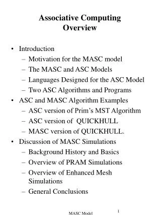
Associative Computing Overview
Associative Computing Overview. Introduction Motivation for the MASC model The MASC and ASC Models Languages Designed for the ASC Model Two ASC Algorithms and Programs ASC and MASC Algorithm Examples ASC version of Prim’s MST Algorithm ASC version of QUICKHULL

Associative Computing Overview
E N D
Presentation Transcript
Associative Computing Overview • Introduction • Motivation for the MASC model • The MASC and ASC Models • Languages Designed for the ASC Model • Two ASC Algorithms and Programs • ASC and MASC Algorithm Examples • ASC version of Prim’s MST Algorithm • ASC version of QUICKHULL • MASC version of QUICKHULL. • Discussion of MASC Simulations • Background History and Basics • Overview of PRAM Simulations • Overview of Enhanced Mesh Simulations • General Conclusions MASC Model
Associative Computing References Note: KSU papers listed are available on the website www.cs.kent.edu/~parallel/ • Maher Atwah, Johnnie Baker, and Selim Akl, An Associative Implementation of Classical Convex Hull Algorithms, Proc of the IASTED International Conference on Parallel and Distributed Computing and Systems, 1996, 435-438 • Johnnie Baker and Mingxian Jin, Simulation of Enhanced Meshes with MASC, a MSIMD Model, Proc. of the Eleventh IASTED International Conference on Parallel and Distributed Computing and Systems, Nov. 1999, 511-516. • Mingxian Jin, Johnnie Baker, and Kenneth Batcher, Timings for Associative Operations on the MASC Model, Proc. of the 15th International Parallel and Distributed Processing Symposium, (Workshop on Massively Parallel Processing, San Francisco, April 2001. • Jerry Potter, Johnnie Baker, Stephen Scott, Arvind Bansal, Chokchai Leangsuksun, and Chandra Asthagiri, An Associative Computing Paradigm, Special Issue on Associative Processing, IEEE Computer, 27(11):19-25, Nov. 1994. (Note: MASC is called ‘ASC’ in this article.) • Jerry Potter, Associative Computing - A Programming Paradigm for Massively Parallel Computers, Plenum Publishing Company, 1992 MASC Model
Associative Computing Associative Computers: A SIMD computers with certain additional features supported in hardware. • These additional features can be supported (less efficiently) in traditional SIMDs in software. • The name “associative” is due to its ability to locate items in the memory of PEs by content rather than location. The ASC model (for ASsociative Computing) gives a list of the properties assumed for an associative computer. The MASC (for Multiple ASC) Model • Supports multiple SIMD (or MSIMD) computation. • Allows model to have more than one Instruction Stream (IS) • The IS corresponds to the control unit of a SIMD. • ASC is the MASC model with only one IS. • The one IS version of the MASC model is sufficiently important to have its own name. MASC Model
Motivation For MASC Model • The STARAN Computer (Goodyear Aerospace, early 1970’s) provided an architectural model for associative computing. • MASC provides a ‘definition’ for associative computing. • Associative computing extends the data parallel paradigm to a complete computational model. • Provides a platform for developing and comparing associative, MSIMD (Multiple SIMD) type programs. • MASC is studied locally as a computational model (Baker), programming model (Potter), and architectural model (Baker, Potter, & Walker). • Provides a practical model that supports massive parallelism. • Model can also support intermediate parallel applications (e.g., multimedia computation, interactive graphics) using on-chip technology. • Model addresses fact that most parallel applications are data parallel in nature, but contain several regions where significant branching occurs. • Normally, at most eight active sub-branches in practical applications. • Provides a hybrid data-parallel, control-parallel model that can be compared to other models. MASC Model
Basic Components • An array of cells, each consisting of a simple PE (or enhanced ALU) and its local memory • An interconnection network between the cells • One or more instruction streams (ISs) • An IS communications network • MASC is a MSIMD model that supports • both data and control parallelism • associative programming. • MASC(n, j) is a MASC model with n PEs and j ISs MASC Model
Basic Properties of MASC • Reference: Paper by [Potter, Baker, et. al.] • Instruction Streams or ISs • Logically a processor with a bus to each cell • Each IS has a copy of the program and can broadcast instructions to cells in unit time • NOTE: MASC(n,1) is called ASC • Cell Properties • Each cell consists of a PE and its local memory • All cells listen to only one IS • Cells can switch ISs in unit time, based on a data test. • A cell can be active, inactive, or idle • Inactive cells listen but do not execute IS commands until reactivated • Idle cells contain no essential data and are available for reassignment • Responder Processing • An IS can detect if a data test is satisfied by any of its responder cells in constant time (i.e., any-responders?). • An IS can select an arbitrary responder in constant time (i.e., pick-one). • Justified by implementations using a resolver in paper by Jin, Baker, & Batcher. MASC Model
Constant Time Global Operations (across PEs with a common IS) • Logical OR and AND of binary values • Maximum and minimum of numbers • Associative searches (see next slide) • Communications • There are three real or virtual networks • PE communications network • IS broadcast/reduction network • IS communications network • Communications can be supported by various techniques • actual networks such as 2D mesh • bus networks • shared memory • Control Features • PEs, ISs, and networks all operate synchronously, using the same clock • Restricted control parallelism used to coordinate the multiple ISs. Observation: The ASC properties that are unusual for SIMDs are the constant time operations: • Constant time responder processing • Constant time global operations MASC Model
Busy- idle On lot Color Model Price Year Make PE1 1 red Dodge 1 1994 0 PE2 0 PE3 1 blue 1996 Ford 1 IS PE4 0 1 1998 white Ford PE5 0 0 PE6 0 0 1 1 Subaru PE7 1997 red The Associative Search MASC Model
Characteristics of Associative Programming • Consistent use of data parallel programming • Consistent use of global associative searching & responder processing • Usually, frequent use of the constant time global reduction operations: AND, OR, MAX, MIN • Broadcast of data using IS bus (and IS fork and join operations for MASC) allows the use of the PE network to be restricted to parallel data movement. • Tabular representation of data • Use of searching instead of sorting • Use of searching instead of pointers • Use of searching instead of the ordering provided by linked lists, stacks, queues • Promotes an highly intuitive programming style that promotes high productivity • Uses structure codes (i.e., numeric representation) to represent data structures such as trees, graphs, embedded lists, and matrices. • See Nov. 1994 IEEE Computer article. • Also, see “Associative Computing” book by Potter. MASC Model
Languages Designed for MASC • The ASC language was designed by Jerry Potter for MASC(n,1) (or ASC). • Based on C and Pascal • Initially designed as a parallel language. • Avoids compromises required to extend an existing sequential language • E.g., avoids unneeded sequential constructs such as pointers • Implemented on several SIMD computers • Goodyear Aerospace’s STARAN • Goodyear/Loral’s ASPRO • Thinking Machine’s CM-2 • WaveTracer • ACE is a higher level language that uses natural language syntax; e.g., plurals, pronouns. • Anglish is an ACE variant that uses an English-like grammar (e.g., “their”, “its”) • An OOPs version of ASC for MASC(n,k) is planned (by Potter and his students) • Language References: • ASC Primer • “Associative Computing” book by Potter [11] • Potter’s website: www.cs.kent.edu/~potter • Websites identified on the class website MASC Model
Algorithms and Programs Implemented in ASC • A wide range of algorithms implemented in ASC without use of PE network • Graph Algorithms • minimal spanning tree • shortest path • connected components • Computational Geometry Algorithms • convex hull algorithms (Jarvis March, Quickhull, Graham Scan, etc) • Dynamic hull algorithms • String Matching Algorithms • all exact substring matches • all exact matches with “don’t care” (i.e., wild card) characters. • Algorithms for NP-complete problems • traveling salesperson • 2-D knapsack. • Data Base Management Software • associative data base • relational data base MASC Model
(Cont) ASC Algorithms and Programs • A Two Pass Compiler for ASC • first pass • optimization phase • Two Rule-Based Inference Engines • OPS-5 interpreter • PPL (Parallel Production Language interpreter) • A Context Sensitive Language Interpreter • (OPS-5 variables force context sensitivity) • An associative PROLOG interpreter • Numerous Programs in ASC using a PE network • 2-D Knapsack Algorithm using a 1-D mesh • Image Processing algorithms using 1-D mesh • FFT using Flip Network • Matrix Multiplication using 1-D mesh • An Air Traffic Control Program (using Flip network connecting PEs to memory) • Demonstrated using live data at Knoxville in mid 70’s. MASC Model
Preliminaries for ASC Algorithm for MST • Next, a “data structure” level presentation of Prim’s algorithm for the MST is given. • The data structure used is illustrated in the next two slides. • This example is from the Nov. 1994 IEEE Computer paper cited in the references. • There are two types of variables for the ASC model, namely • the parallel variables (i.e., ones for the PEs) • the scalar variables (ie., the ones used by the control unit). • Scalar variables are essentially global variables. • Can replace each with a parallel variable. • In order to distinguish between them here, the parallel variables names end with a “$” symbol. • Each step in this algorithm is constant. • One MST edge is selected during each pass through the loop in this algorithm. • Since a spanning tree has n-1 edges, the running time of this algorithm is O(n) and its cost is O(n 2). • Since the sequential running time of the Prim MST algorithm is O(n 2) and is time optimal, this parallel implementation is cost optimal. MASC Model
a 2 2 8 7 b c 4 3 9 6 e d 3 f Figure 6 in [Potter, Baker, et. al.] MASC Model
candidate$ current_best$ mask$ node$ parent$ PEs d$ c$ b$ e$ f$ a$ a ∞ 2 8 ∞ ∞ ∞ no b 2 ∞ 7 4 3 ∞ no a 2 c 8 7 ∞ ∞ 6 9 yes b 7 IS sequential program control d ∞ 4 ∞ ∞ 3 ∞ yes b 4 a e ∞ 3 6 3 ∞ ∞ yes b 3 root b f ∞ ∞ 9 ∞ ∞ ∞ wait next- node MASC Model
Algorithm: ASC-MST-PRIM(root) • Initialize candidates to “waiting” • If there are any finite values in root’s field, • set candidate$ to “yes” • set parent$ to root • set current_best$ to the values in root’s field • set root’s candidate field to “no” • Loop while some candidate$ contain “yes” • for them • restrict mask$ to mindex(current_best$) • set next_node to a node identified in the preceding step • set its candidate to ‘no” • if the values in next_node’s field are less than current_best$, then • set current_best$ to value in next_node’s field • set parent$ to next_node • if candidate$ is “waiting” and the value in next_node’s field is finite • set candidate$ to “yes” • set parent$ to next_node • set current_best to the values in next_node’s field Figure 6(c) in [10, Potter, Baker, et. al.] MASC Model
Comments on Figure 6 • The three preceding slides show figure 6 from the [Potter, Baker, et.al.] IEEE Computer, Nov 1994]. • Figure 6c gives a compact, data-structures level pseudo-code description for this algorithm • Pseudo-code illustrates Potter’s use of pronouns (e.g., them) and possessive nouns. • The mindex function returns the index of a processor holding the minimal value. • This MST pseudo-code is much shorter and simpler than data-structure level sequential MST pseudo-codes • e.g., see one of Baase’s textbook cited below • Algorithm given in Baase’s books is essentially the same as this parallel algorithm • Next, a more detailed explanation of the algorithm in Figure 6c will be given. Reference: Sara Baase, Computer Algorithms: Introduction to Design and Analysis, 2nd Edition, Addison Wesley Publishing Co.,1988, 162-166. (Alternately, see the 3rd edition by Baase & Van Gelder, 2000.) MASC Model
Algorithm: ASC-MSP-PRIM • Initially assign any node to root. • All processors set • candidate$ to “waiting” • current-best$ to • the candidate fieldfor the root node to “no” • All processors whose distance d from their node to root node is finite do • Set their candidate$ field to “yes • Set their parent$ field to root. • Set current_best$ = d. • While the candidate field of some processor is “yes”, • Restrict the active processors to those responding and (for these processors) do • Compute the minimum value x of current_best$. • Restrict the active processors to those with current_best$ = x and do • pick an active processor, say one that contains node y. • Set the candidate$ value of node y to “no” • Set the scalar variable next-node to y. MASC Model
If the value z in the next_node column of a processor is less than its current_best$ value, then • Set current_best$ to z. • Set parent$ to next_node • For all processors, if candidate$ is “waiting” and the distance of its node from next_node is not , then • Set candidate$ to “yes” • Set parent$ to next-node • Set current_best$ to the distance of its node from next_node. MASC Model
h e w Quickhull Algorithm for ASC • Reference: • [Maher, et.al, Associative Convex Hull] • Review of Sequential Quickhull Algorithm • Suffices to find the upper convex hull of points in below diagram that are on or above line • Select point h so that the area of triangle weh is maximal. • Proceed recursively with the sets of points on or above the lines and . MASC Model
point$ y-coord$ left-point$ x-coord$ right-pt$ job$ area$ name$ hull$ p1 1 3 p1 p3 1 1 w 0 p2 7 1 p1 p3 0 IS 12 2 p1 p3 1 1 e p3 p4 8 4 p1 p3 1 p5 11 7 p1 p3 1 h ctr h p6 8 9 p1 p3 1 1 p7 2 6 p1 p3 1 P6, h p5 p7 p4 p1, w P3, e p2 MASC Model
ASC Quickhull Algorithm(Upper Convex Hull) ASC-Quickhull( planar-point-set ) • Initialize: ctr = 1, area$ = 0, hull$ = 0 • Find the PE with the minimal x-coord$ and let w be its point$ • Set its hull$ value to 1 • Find the PE with the PE with maximal x-coord$ and let e be its point$ • Set its hull$ to 1 • All PEs set their left-pt to w and right-pt to e. • If the point$ for a PE lies above the line • Then set its job$ value to 1 • Else set its job$ value to 0 MASC Model
ASC Quickhull (continued) • Loop while parallel job$ contains a nonzero value • The IS makes its active cell those with a maximal job$ value. • Each active PE stores in area$ the area of triangle( left-pt$, right-pt$, point$ ) • Find the PE with the maximal area$ and let h be its point. • Set its hull$ value to 1 • Each active PE whose point$ is above sets its job$ value to ++ctr • Each active PE whose point$ is above sets its job$ to ++ctr • Each active PE with job$ < ctr -2 sets its job$ value to 0 MASC Model
Performance of ASC-Quickhull Average Case: • Assume • Roughly 1/3 of the points above each line being processed are eliminated. • O(lg n) points are on the convex hull. • Then the average running time is O(lg n) • The average cost is O(n lg n) Worst Case: • Running time is O(n). • Cost is O(n2) 5 3 1 4 2 6 0 MASC Model
2 2 1 1 2 2 0 MASC Quickhull Algorithm(Upper Convex Hull) Algorithm: • Use IS1 to execute the first loop of ASC-Quickhull • Idle ISs request problems from busy ISs who have inactive jobs on their job$ list. • Control of the PEs for an inactive job are transferred to the idle IS. The control of these PEs is returned to original IS after the job is finished. MASC Model
Analysis for MASC Quicksort Average Case: • Assumptions: • roughly 1/3 of the points above each line being processed are eliminated. • O(lg n) Instruction Streams are available. • There are O(lg n) convex hull points • The average running time is O(lg lg n) • Essentially constant time for real world problems. Worst Case • O(n) Note: Taken from a latex presentation prepared by Atwah called “An Associative Model of Computation” in directory ~jbaker/slides/matwah. MASC Model
MASC SIMULATION RESULTS • Remaining slides in this chapter were covered very quickly and lightly in F04 • They were not tested. • Expect this material to be covered primarily in parallel algorithms course MASC Model
Previous MASC Simulation(See Preceding Slide) • MASC Simulation of PRAM • MASC(n,j) can simulate priority CRCW PRAM(n,m) in O(min{n/j, m/j}) with high probability. • MASC(n,1) [or ASC] can simulate priority CRCW with a constant number of global memory locations in constant time • This result is stronger than it first appears • Some CRCW algorithms only require a constant nr of global memory locations • A reverse simulation of MASC by Combining CRCW PRAM result will be in the dissertation of Mingxian Jin • Self-simulation of MASC • Provides an efficient algorithm for MASC to efficiently simulate a larger MASC - with more PEs and/or ISs. • Establishes that MASC is highly scalable • MASC(n,j) can simulate MASC(N,J) in O(N/n + J) extra time and O(N/n + J) extra memory. MASC Model
The Enhanced Mesh, MMB • References: • [Baker & Jin], Reference listed on Slide 19 • Mingxian Jin, Evaluating the power of the parallel MASC model using simulations and Real-Time Applications, KSU Dissertation Aug. 2004,145 pages. • Enhanced meshes are basic mesh models augmented with fixed or reconfigurable buses • At most one PE on a bus can broadcast to remaining PEs during one step. • Best-known fixed bus example: • Mesh with multiple broadcasting (MMB) • Standard 2-D mesh • Row and column bus enhancements • Broadcasts can occur along only row or column buses (but not both) in one step MASC Model
The Reconfigurable Enhanced Mesh RM • For all reconfigurable bus models, buses are created dynamically during execution • Best known example: • General Reconfigurable Mesh (RM) • Each PE has four ports called N,S, E, W (often called “NEWS”) • In one step, each PE can set the connections of its ports, based on local data • At most two disjoint pairs of ports can be connected at any time • One such connection is the adjacent pairs, {{N,E}, {W,S}}. MASC Model
Simulation Preliminaries • Reasons to simulate other models using MASC • Allows a better understanding of the power of MASC • Provides a simulation algorithm that can be used to convert algorithms designed for the other model to MASC • Basic Assumption Used in the Simulations • MASC(n, ) has a mesh PE network with row-major ordering • The enhanced meshes have a 2D mesh with the same size and ordering • Each PE in MASC has the same computational power as an enhanced mesh PE • The MASC buses and the buses of the enhanced mesh have the same characteristics • The word lengths of both models are the same and at least lg(n). • Each PE in MASC knows its position in the 2D mesh. • Words can store the positions of various PEs MASC Model
Simulation Mappings between MASC & the Enhanced Mesh MMB • The mapping is between MASC(n, ) and Enhanced meshes of size • The mapping assigns a PE in one model to the PE that is in the same position in the 2D mesh in the other model • The ith IS in MASC simulates both the ith row and the ith column buses MASC Model
Simulation of MMB with MASC • Since both models have identical 2D meshes, these do not need to be simulated • Since the power of PEs in respective models are identical, their local computations are not simulated • To simulate a MMB row broadcast on the MASC, • All PEs switch to their assigned row IS • The IS for each row checks to see if there is a PE that wishes to broadcast • If true, the IS broadcasts this value to all of its PEs (i.e., the ones on its assigned row). • Simulation of a MMB column broadcast is similar • The running time is O(1) • There are examples that show the MASC model is strictly more powerful than the MMB model Theorem 1. • MASC(n, j) with a 2-D mesh is strictly more powerful than a MMB for j = ( ). • An algorithm for a MMB can be executed on MASC(n, j) with j=( ) and a 2-D mesh with a running time at least fast as the MMB time. MASC Model
Simulation of MASC by MMB • PE(1,1) stores a copy of the program and simulates the ISs sequentially. • Each instruction stream command or datum is first sent by P(1,1) to the PEs in the first column. • Next, the PEs in the first column broadcast this command or datum along the rows to all PEs. • Each MMB processor uses two registers, channel and status, to decide whether or not to execute the current instruction. • channel records which IS the processor is assigned to • status records whether PE is active, inactive, idle • The simulation of simultaneous broadcasts of ISs takes O( ) time. • A local computation, memory access, or a data movement along local links are identical in the two models and require O(1) time. • The execution of a global reduction operator OR, AND, MAX, MIN takes O( ) using an optimal MMB algorithm (details omitted). • Since the global reduction operators may be computed for O( ) ISs, an upper bound is O( ) or O( ). Theorem 3. • MASC(n, ) with a 2-D mesh can be simulated by a MMB in O( ) time with O( ) extra memory MASC Model
Simulation Conclusions • MASC is strictly more powerful than an MMB of the same size. • Any algorithm for an MMB can be executed on a MASC of the same size with the same running time. In particular, • Optimal algorithms for MMB are also optimal when executed on MASC • CLAIM: MASC and RM are very dissimilar and can not simulate each other efficiently. • Details in Jin’s dissertation. MASC Model
Suggested Changes • Probably move simulation material to the parallel algorithms course. MASC Model