Introduction to Finite Element Method (FEM)

1. Introduction to Finite Element Method (FEM) Chapter 9 Lecture Notes Mohd Sani Mohamad Hashim Universiti Malaysia Perlis ENT 258 Numerical Analysis

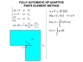
2. Introduction FEA or sometimes referred as FEM, has become a powerful tool for numerical solution of a wide range of engineering problems. FEA is a computational technique used to obtain approximate solutions of boundary value problems. Example applications of FEA: Deformation & stress analysis of automotive, aircraft, building and bridge structures. Field analysis of heat flux, fluid flow, magnetic flux, seepage and other flow problems. Research about its application is still open to non-engineering fields such as economic analysis, optimization, etc. 2

3. Introduction Relationship between CAD, CAE and CAM. CAE CAD CAA CAM • With the advances in computer technology and CAD systems, complex problems can be modelled relative ease & accurate. 3

4. Introduction

5. Fundamental Concepts The concept of FEA In this method, a complex region defining a continuum is discretized into simple geometric shapes called finite elements The material properties, and the governing relationships are considered over these elements and expressed in terms of unknown values at element corners An assembly process, considering the loading and constraints, results in a set of equations. 5

6. One-dimensional Problems In one dimensional problems, every node is permitted to displace only in the ±xdirection. Each node has only one degree of freedom (dof). Element division, numbering scheme. 6

7. One-dimensional Problems Potential-Energy Approach Assembly of the global stiffness matrix and load vector:

8. One-dimensional Problems PENALTY APPROACH The modified stiffness matrix and modified load vector are given by: It is that the value of C is: Reaction force: R = -CQ 8

9. One-dimensional Problems Example 1: Consider the bar shown in fig. E3.4. An axial load P = 200x103 N is applied as shown. Using the penalty approach for handling boundary conditions do the following: (a) Determine the nodal displacements (b) Determine the stress in each material (c) Determine the reaction forces 9

10. One-dimensional Problems 300 mm 400 mm P 1 3 2 1 2 Aluminum A1 = 2400 mm2 E1 = 70 x 109 N/m2 Steel A2 = 600 mm2 E2 = 200 x 109 N/m2 10

11. Example 1 • (a) Determine the nodal displacements 1 2 Global dof 1 2 2 3 2 3 11 11

12. Example 1 • Structural stiffness matrix K is assembled from k1 and k2 • Global load vector 12 12

13. Example 1 • Global load vector is • dofs 1 and 3 are fixed • Using penalty approach, a large number of C is added to the first and third diagonal element of K max 13 13

14. Example 1 • Finite element equation are given by 14 14

15. Example 1 • The solution of displacement 15 15

16. Example 1 • (b) the stresses in each element • Using Eq. 3.15 and Eq. 3.16 16 16

17. (c) Determine the reaction force at the support Using Eq. 3.78 Example 1 17

18. One-dimensional Heat Conduction The governing equation for one-dimensional heat conduction in steady-state: Boundary conditions: 18

19. One-dimensional Heat Conduction After integration and substitution, we have: The global matrices KT and R are assembled from element matrices kT and rQ, as given in: R is a heat rate vector. C = max|Kij| x 104 19

20. One-dimensional Heat Conduction Example 2: 20

21. One-dimensional Heat Conduction Solution: The element and global conductivity matrices are: Heat rate vector, R consists only of hT∞ 21

22. One-dimensional Heat Conduction Solution: Choose C based on Using penalty approach 22