Efficient Methods for Data Cube Computation

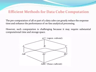
1. Efficient Methods for Data Cube Computation The pre-computation of all or part of a data cube can greatly reduce the response time and enhance the performance of on-line analytical processing. However, such computation is challenging because it may require substantial computational time and storage space.

2. Cube Materialization: Full Cube, Iceberg Cube, Closed Cube, and Shell Cube A data cube is a lattice of cuboids. Each cuboid represents a group-by. ABC is the base cuboid, containing all three of the dimensions. Here, the aggregate measure, M, is computed for each possible combination of the three dimensions. The base cuboid is the least generalized of all of the cuboids in the data cube. The most generalized cuboid is the apex cuboid, commonly represented as all. It contains one value—it aggregates measure M for all of the tuples stored in the base cuboid. To drill down in the data cube, we move from the apex cuboid, downward in the lattice. To roll up, we move from the base cuboid, upward

3. Cube Materialization: Full Cube, Iceberg Cube, Closed Cube, and Shell Cube A cell in the base cuboid is a base cell. A cell from a nonbase cuboid is an aggregate cell. An aggregate cell aggregates over one or more dimensions, where each aggregated dimension is indicated by a * in the cell notation. Suppose we have an n-dimensional data cube. Let a = (a1, a2, . . . , an, measures) be a cell from one of the cuboids making up the data cube. We say that a is an m-dimensional cell (that is, from an m-dimensional cuboid) if exactly m (m <= n) values among {a1, a2, : : : , an} are not *. If m = n, then a is a base cell; otherwise, it is an aggregate cell (i.e., where m < n).

4. Cube Materialization: Full Cube, Iceberg Cube, Closed Cube, and Shell Cube • Consider a data cube with the dimensions month, city, and customer group, and the measure price. • (Jan, * , * , 2800) and (*, Toronto, * , 1200) are 1-D cells, (Jan, * , Business, 150) is a 2-D cell, and (Jan, Toronto, Business, 45) is a 3-D cell. • An ancestor-descendant relationship may exist between cells. • In an n-dimensional data cube, an i-D cell a = (a1, a2, . . . , an, measuresa) is an ancestor of a j-D cell b = (b1, b2, . . . , bn, measuresb), and b is a descendant of a, if and only if • (1) i < j, and • (2) for 1 <=m<=n, am = bm whenever am *. • In particular, cell a is called a parent of cell b, and b is a child of a, if and only if j = i+1 and b is a descendant of a.

5. Cube Materialization: Full Cube, Iceberg Cube, Closed Cube, and Shell Cube Referring to our previous example, 1-D cell a=(Jan, * , * , 2800), and 2-D cell b = (Jan, * , Business, 150), are ancestors of 3-D cell c = (Jan, Toronto, Business, 45); c is a descendant of both a and b. bis a parent of c, and c is a child of b. In order to ensure fast on-line analytical processing, it is sometimes desirable to pre-compute the full cube. This, however, is exponential to the number of dimensions. That is, a data cube of n dimensions contains 2n cuboids. There are even more cuboids if we consider concept hierarchies for each dimension. In addition, the size of each cuboid depends on the cardinality of its dimensions. Thus, pre-computation of the full cube can require huge and often excessive amounts of memory.

6. Cube Materialization: Full Cube, Iceberg Cube, Closed Cube, and Shell Cube Partial materialization of data cubes offers an interesting trade-off between storage space and response time for OLAP. Instead of computing the full cube, we can compute only a subset of the data cube’s cuboids, or subcubes consisting of subsets of cells from the various cuboids. Many cells in a cuboid may actually be of little or no interest to the data analyst. Recall that each cell in a full cube records an aggregate value. Measures such as count, sum, or sales in dollars are commonly used. For many cells in a cuboid, the measure value will be zero. When the product of the cardinalities for the dimensions in a cuboid is large relative to the number of nonzero-valued tuples that are stored in the cuboid, then we say that the cuboid is sparse. If a cube contains many sparse cuboids, we say that the cube is sparse.

7. Cube Materialization: Full Cube, Iceberg Cube, Closed Cube, and Shell Cube In many cases, a substantial amount of the cube’s space could be taken up by a large number of cells with very low measure values. This is because the cube cells are often quite sparsely distributed within a multiple dimensional space. For example, a customer may only buy a few items in a store at a time. Such an event will generate only a few nonempty cells, leaving most other cube cells empty. In such situations, it is useful to materialize only those cells in a cuboid (group-by) whose measure value is above some minimum threshold.

8. Cube Materialization: Full Cube, Iceberg Cube, Closed Cube, and Shell Cube In a data cube for sales, say, we may wish to materialize only those cells for which count is 10 or only those cells representing sales $100. This not only saves processing time and disk space, but also leads to a more focused analysis. The cells that cannot pass the threshold are likely to be too trivial to warrant further analysis. Such partially materialized cubes are known as iceberg cubes. The minimum threshold is called the minimum support threshold, or minimum

9. Cube Materialization: Full Cube, Iceberg Cube, Closed Cube, and Shell Cube An iceberg cube can be specified with an SQL query, as shown in the following example. compute cube sales iceberg as select month, city, customer group, count(*) from salesInfo cube by month, city, customer group having count(*) >= min sup The compute cube statement specifies the precomputation of the iceberg cube, sales iceberg, with the dimensions month, city, and customer group, and the aggregate measure count(). The input tuples are in the salesInfo relation. The cube by clause specifies that aggregates (group-by’s) are to be formed for each of the possible subsets of the given dimensions.