Advanced Compiler Techniques
Advanced Compiler Techniques. Data Flow Analysis. LIU Xianhua School of EECS, Peking University. REVIEW. Introduc tion to optimization Control Flow Analysis Basic knowledge Basic blocks Control-flow graphs Local Optimizations Peephole optimizations. Outline. Some Basic Ideas

Advanced Compiler Techniques
E N D
Presentation Transcript
Advanced Compiler Techniques Data Flow Analysis LIU Xianhua School of EECS, Peking University
REVIEW • Introduction to optimization • Control Flow Analysis • Basic knowledge • Basic blocks • Control-flow graphs • Local Optimizations • Peephole optimizations “Advanced Compiler Techniques”
Outline • Some Basic Ideas • Reaching Definitions • Available Expressions • Live Variables “Advanced Compiler Techniques”
Levels of Optimizations • Local • inside a basic block • Global (intraprocedural) • Across basic blocks • Whole procedure analysis • Interprocedural • Across procedures • Whole program analysis “Advanced Compiler Techniques”
Dataflow Analysis • Last lecture: • How to analyze and transform within a basic block • This lecture: • How to do it for the entire procedure “Advanced Compiler Techniques”
An Obvious Theorem boolean x = true; while (x) { . . . // no change to x } • Doesn’t terminate. • Proof: only assignment to x is at top, so x is always true. x = true if x == true “body” “Advanced Compiler Techniques”
Formulation: Reaching Definitions d2 d1 • Each place some variable x is assigned is a definition. • Ask: for this use of x, where could x last have been defined. • In our example: only at x=true. d1: x = true d1 d2 if x == true d1 d2: a = 10 “Advanced Compiler Techniques”
Clincher • Since at x == true, d1 is the only definition of x that reaches, it must be that x is true at that point. • The conditional is not really a conditional and can be replaced by a jump. “Advanced Compiler Techniques”
Not Always That Easy int i = 2; intj = 3; while (i != j) { if (i < j) i += 2; else j += 2; } “Advanced Compiler Techniques”
Not Always That Easy d1 d2 d3 d4 d2, d3, d4 d1, d3, d4 d1, d2, d3, d4 d1, d2, d3, d4 • Build the Flow Graph d1: i = 2 d2: j = 3 if i != j d1, d2, d3, d4 if i < j d3: i = i+2 d4: j = j+2 “Advanced Compiler Techniques”
DFA Is Sufficient Only • In this example, i can be defined in two places, and jin two places. • No obvious way to discover that i!=j is always true. • But OK, because reaching definitions is sufficient to catch most opportunities for constant folding (replacement of a variable by its only possible value). “Advanced Compiler Techniques”
Be Conservative! • (Code optimization only) • It’s OK to discover a subset of the opportunities to make some code-improving transformation. • It’s notOK to think you have an opportunity that you don’t really have. “Advanced Compiler Techniques”
Example: Be Conservative Another def of x d2 boolean x = true; while (x) { . . . *p = false; . . . } • Is it possible that ppoints to x? d1: x = true d1 if x == true d2: *p = false “Advanced Compiler Techniques”
Possible Resolution • Just as data-flow analysis of “reaching definitions” can tell what definitions of x might reach a point, another DFA can eliminate cases where p definitely does not point to x. • Example: the only definition of pis p = &y and there is no possibility that y is an alias of x. “Advanced Compiler Techniques”
Data-Flow Analysis Schema • Data-flow value: at every program point • Domain: The set of possible data-flow values for this application • IN[S] and OUT[S]: the data-flow values before and after each statement s • Data-flow problem: find a solution to a set of constraints on the IN [s] ‘s and OUT[s] ‘s, for all statements s. • based on the semantics of the statements ("transfer functions" ) • based on the flow of control. “Advanced Compiler Techniques”
Data-Flow Equations (1) • A statement/basic block can generate a definition. • A statement/basic block can either • Kill a definition of x if it surely redefines x. • Transmit a definition if it may not redefine the same variable(s) as that definition. “Advanced Compiler Techniques”
Data-Flow Equations (2) • Variables: • IN[s] = set of data flow values the before a statement s. • OUT[s]= set of data flow values the after a statement s. • Extends: • IN[B] = set of definitions reaching the beginning of block B. • OUT[B] = set of definitions reaching the end of B. “Advanced Compiler Techniques”
Data-Flow Equations (3) • Two kinds of Constraints: Transfer Functions: OUT[s] = fs(IN[s]) IN[s] = fs(OUT[s]) reversed~ Control Flow Constraints: If B consists of statements s1,s2,…,sn IN[si+1] = OUT[si] “Advanced Compiler Techniques”
Between Blocks • Forward analysis(eg: Reaching definitions) • Transfer equations • OUT[B] = fB(IN[B]) Where fB = fsn◦ ••• ◦ fs2 ◦ fs1 • Confluence equations • IN[B] = UP a predecessor of B OUT[P] • Backward analysis(eg: live variables) • Transfer equations • IN[B] = fB (OUT[B]) • Confluence equations • OUT[B] = US a successor of B IN[S]. “Advanced Compiler Techniques”
Confluence Equations {d1, d2} {d2, d3} • IN(B) = ∪predecessor P of B OUT(P) • OUT(B) = ∪successor S of B IN(S) P1 P2 {d1, d2, d3} B “Advanced Compiler Techniques”
Transfer Equations • OUT[B] = fB(IN[B]) • IN[B] = fB(OUT[B]) ~reverse • Generate a definition in the block if its variable is not definitely rewritten later in the basic block. • Kill a definition if its variable is definitely rewritten in the block. “Advanced Compiler Techniques”
Example: Gen and Kill • An internal definition may be both killed and generated. • For any block B: OUT(B) = (IN(B) – Kill(B)) ∪Gen(B) IN = {d2(x), d3(y), d3(z), d5(y), d6(y), d7(z)} Kill includes {d2(x), d3(y), d5(y), d6(y),…} d1: y = 3 d2: x = y+z d3: *p = 10 d4: y = 5 Gen = {d2(x), d3(x), d3(z),…, d4(y)} OUT = {d2(x), d3(x), d3(z),…, d4(y), d7(z)} “Advanced Compiler Techniques”
Iterative Solution to Equations • For an n-block flow graph, there are 2n equations in 2n unknowns. • Alas, the solution is not unique. • Standard theory assumes a field of constants; sets are not a field. • Use iterative solution to get the least fixed-point. • Identifies any def that might reach a point. “Advanced Compiler Techniques”
Example: Reaching Definitions IN(B1) = {} OUT(B1) = { IN(B2) = { d1, OUT(B2) = { IN(B3) = { d1, OUT(B3) = { d1: x = 5 B1 d1} d2} if x == 10 B2 d1, d2} d2} d2: x = 15 B3 d2} “Advanced Compiler Techniques”
Outline • Some Basic Ideas • Reaching Definitions • Available Expressions • Live Variables “Advanced Compiler Techniques”
Reaching Definitions • Concept of definition and use • a = x+y is a definition of a is a use of x and y • A definition reaches a use if value written by definition may be read by use “Advanced Compiler Techniques”
Reaching Definitions s = 0; a = 4; i = 0; k == 0 b = 1; b = 2; i < n s = s + a*b; i = i + 1; return s “Advanced Compiler Techniques”
Reaching Def. and Const. Propagation • Is a use of a variable a constant? • Check all reaching definitions • If all assign variable to same constant • Then use is in fact a constant • Can replace variable with constant “Advanced Compiler Techniques”
s = 0; a = 4; i = 0; k == 0 b = 1; b = 2; i < n s = s + a*b; i = i + 1; return s Is a Constant in s = s+a*b? Yes! On all reaching definitions a = 4 “Advanced Compiler Techniques”
s = 0; a = 4; i = 0; k == 0 b = 1; b = 2; i < n s = s + 4*b; i = i + 1; return s Constant Propagation Transform Yes! On all reaching definitions a = 4 “Advanced Compiler Techniques”
s = 0; a = 4; i = 0; k == 0 b = 1; b = 2; i < n s = s + a*b; i = i + 1; return s Is b Constant in s = s+a*b? No! One reaching definition with b = 1 One reaching definition with b = 2 “Advanced Compiler Techniques”
s = 0; a = 4; i = 0; k == 0 s = 0; a = 4; i = 0; k == 0 b = 1; b = 2; i < n b = 1; b = 2; i < n i < n s = s + a*b; i = i + 1; return s s = s + a*b; i = i + 1; s = s + a*b; i = i + 1; return s return s SplittingPreserves Information Lost At Merges “Advanced Compiler Techniques”
s = 0; a = 4; i = 0; k == 0 b = 1; b = 2; i < n s = s + a*b; i = i + 1; return s SplittingPreserves Information Lost At Merges s = 0; a = 4; i = 0; k == 0 b = 1; b = 2; i < n i < n s = s + a*1; i = i + 1; s = s + a*2; i = i + 1; return s return s “Advanced Compiler Techniques”
Computing Reaching Definitions • Compute with sets of definitions • represent sets using bit vectors • each definition has a position in bit vector • At each basic block, compute • definitions that reach start of block • definitions that reach end of block • Do computation by simulating execution of program until reach fixed point “Advanced Compiler Techniques”
1 2 3 4 5 6 7 0000000 1: s = 0; 2: a = 4; 3: i = 0; k == 0 1110000 1 2 3 4 5 6 7 1 2 3 4 5 6 7 1110000 1110000 4: b = 1; 5: b = 2; 1111000 1110100 1 2 3 4 5 6 7 1111100 1111111 i < n 1111100 1111111 1 2 3 4 5 6 7 1 2 3 4 5 6 7 1111111 1111100 1111111 1111100 6: s = s + a*b; 7: i = i + 1; return s 1111100 1111111 0101111 “Advanced Compiler Techniques”
Formalizing Reaching Definitions • Each basic block has • IN - set of definitions that reach beginning of block • OUT - set of definitions that reach end of block • GEN - set of definitions generated in block • KILL - set of definitions killed in block • GEN[s = s + a*b; i = i + 1;] = 0000011 • KILL[s = s + a*b; i = i + 1;] = 1010000 • Compiler scans each basic block to derive GEN and KILL sets “Advanced Compiler Techniques”
Dataflow Equations • IN[b] = OUT[b1] U ... U OUT[bn] • where b1, ..., bn are predecessors of b in CFG • OUT[b] = (IN[b] - KILL[b]) U GEN[b] • IN[entry] = 0000000 • Result: system of equations • KILLB= KILL1 U KILL2 U…U KILLn • GENB=GENn U(GENn-1-KILLn)U (GENn-2-KILLn-1-KILLn) U …U(GEN1-KILL2-KILL3-…-KILLn) “Advanced Compiler Techniques”
Solving Equations • Use fixed point algorithm • Initialize with solution of OUT[b] = 0000000 • Repeatedly apply equations • IN[b] = OUT[b1] U ... U OUT[bn] • OUT[b] = (IN[b] - KILL[b]) U GEN[b] • Until reach fixed point • Until equation application has no further effect • Use a worklist to track which equation applications may have a further effect “Advanced Compiler Techniques”
Reaching Definitions Algorithm for all nodes n in N OUT[n] = emptyset; // OUT[n] = GEN[n]; IN[Entry] = emptyset; OUT[Entry] = GEN[Entry]; Changed = N - { Entry }; // N = all nodes in graph while (Changed != emptyset) choose a node n in Changed; Changed = Changed - { n }; IN[n] = emptyset; for all nodes p in predecessors(n) IN[n] = IN[n] U OUT[p]; OUT[n] = GEN[n] U (IN[n] - KILL[n]); if (OUT[n] changed) for all nodes s in successors(n) Changed = Changed U { s }; “Advanced Compiler Techniques”
Iterative Solution IN(entry) = ∅; for each block B do OUT(B)= ∅; while (changes occur) do for each block B do { IN(B) = ∪predecessors P of B OUT(P); OUT(B) = (IN(B) – Kill(B)) ∪Gen(B); } “Advanced Compiler Techniques”
Example “Advanced Compiler Techniques”
Outline • Some Basic Ideas • Reaching Definitions • Available Expressions • Live Variables “Advanced Compiler Techniques”
Available Expressions • An expression x+y is availableat a point p if • every path from the initial node to p must evaluatex+ybefore reaching p, • and there are no assignments to x or y after the evaluation but before p. • Available Expression information can be used to do global (across basic blocks) CSE • If expression is available at use, no need to reevaluate it “Advanced Compiler Techniques”
Example: Available Expression a = b + c d = e + f f = a + c b = a + d h = c + f g = a + c j = a + b + c + d “Advanced Compiler Techniques”
Is the Expression Available? YES! a = b + c d = e + f f = a + c b = a + d h = c + f g = a + c j = a + b + c + d “Advanced Compiler Techniques”
Is the Expression Available? YES! a = b + c d = e + f f = a + c b = a + d h = c + f g = a + c j = a + b + c + d “Advanced Compiler Techniques”
Is the Expression Available? NO! a = b + c d = e + f f = a + c b = a + d h = c + f g = a + c j = a + b + c + d “Advanced Compiler Techniques”
Is the Expression Available? NO! a = b + c d = e + f f = a + c b = a + d h = c + f g = a + c j = a + b + c + d “Advanced Compiler Techniques”
Is the Expression Available? NO! a = b + c d = e + f f = a + c b = a + d h = c + f g = a + c j = a + b + c + d “Advanced Compiler Techniques”
Is the Expression Available? YES! a = b + c d = e + f f = a + c b = a + d h = c + f g = a + c j = a + b + c + d “Advanced Compiler Techniques”