Static Compiler Optimization Techniques

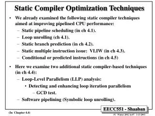
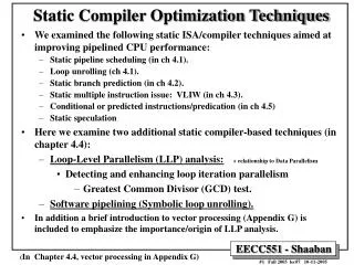
1. Static Compiler Optimization Techniques • We examined the following static ISA/compiler techniques aimed at improving pipelined CPU performance: • Static pipeline scheduling (in ch 4.1). • Loop unrolling (ch 4.1). • Static branch prediction (in ch 4.2). • Static multiple instruction issue: VLIW (in ch 4.3). • Conditional or predicted instructions/predication (in ch 4.5) • Static speculation • Here we examine two additional static compiler-based techniques (in chapter 4.4): • Loop-Level Parallelism (LLP) analysis: • Detecting and enhancing loop iteration parallelism • Greatest Common Divisor (GCD) test. • Software pipelining (Symbolic loop unrolling). • In addition a brief introduction to vector processing (Appendix G) is included to emphasize the importance/origin of LLP analysis. + relationship to Data Parallelism (In Chapter 4.4, vector processing in Appendix G)

2. Data Parallelism & Loop Level Parallelism • Data Parallelism: Similar independent/parallel computations on different elements of arrays that usually result in independent (or parallel) loop iterations when such computations are implemented as sequential programs. • A common way to increase parallelism among instructions is to exploit data parallelism among independent iterations of a loop (e.g exploit Loop Level Parallelism, LLP). • One method covered earlier to accomplish this is by unrolling the loop either statically by the compiler, or dynamically by hardware, which increases the size of the basic block present. This resulting larger basic block provides more instructions that can be scheduled or re-ordered by the compiler/hardware to eliminate more stall cycles. • The following loop has parallel loop iterations since computations in each iterations are data parallel and are performed on different elements of the arrays. for (i=1; i<=1000; i=i+1;) x[i] = x[i] + y[i]; • In supercomputing applications, data parallelism/LLP has been traditionally exploited by vector ISAs/processors, utilizing vector instructions • Vector instructions operate on a number of data items (vectors) producing a vector of elements not just a single result value. The above loop might require just four such instructions. 4 vector instructions: Load Vector X Load Vector Y Add Vector X, X, Y Store Vector X Modified from Loop-unrolling lecture # 3 (3-14-2005)

3. The execution time of the loop has dropped to 14 cycles, or 14/4 = 3.5 clock cycles per element compared to 7 before scheduling and 6 when scheduled but unrolled. Speedup = 6/3.5 = 1.7 Unrolling the loop exposed more computations that can be scheduled to minimize stalls by increasing the size of the basic block from 5 instructions in the original loop to 14 instructions in the unrolled loop. Larger Basic Block More ILP Loop Unrolling Example From Lecture #3 (slide # 10) for (i=1000; i>0; i=i-1) x[i] = x[i] + s; Note: Independent Loop Iterations Resulting from data parallel operations on elements of array X When scheduled for pipeline Loop: L.D F0, 0(R1) L.D F6,-8 (R1) L.D F10, -16(R1) L.D F14, -24(R1) ADD.D F4, F0, F2 ADD.D F8, F6, F2 ADD.D F12, F10, F2 ADD.D F16, F14, F2 S.D F4, 0(R1) S.D F8, -8(R1) DADDUI R1, R1,# -32 S.D F12, 16(R1),F12 BNE R1,R2, Loop S.D F16, 8(R1), F16 ;8-32 = -24 Loop unrolling exploits data parallelism among independent iterations of a loop Loop unrolled four times and scheduled

4. 1 2 3 ….. 1000 Iteration # S1 S1 S1 S1 … Dependency Graph Loop-Level Parallelism (LLP) Analysis • Loop-Level Parallelism (LLP) analysis focuses on whether data accesses in later iterations of a loop are data dependent on data values produced in earlier iterations and possibly making loop iterations independent (parallel). e.g. in for (i=1; i<=1000; i++) x[i] = x[i] + s; the computation in each iteration is independent of the previous iterations and the loop is thus parallel. The use of X[i] twice is within a single iteration. • Thus loop iterations are parallel (or independent from each other). • Loop-carried Data Dependence: A data dependence between different loop iterations (data produced in an earlier iteration used in a later one). • Not Loop-carried Data Dependence: Data dependence within the same loop iteration. • LLP analysis is important in software optimizations such as loop unrolling since it usually requires loop iterations to be independent(and in vector processing). • LLP analysis is normally done at the source code level or close to it since assembly language and target machine code generation introduces loop-carried name dependence in the registers used in the loop. • Instruction level parallelism (ILP) analysis, on the other hand, is usually done when instructions are generated by the compiler. S1 (Body of Loop) (In Chapter 4.4)

5. Loop-carried Dependence i i+1 Iteration # S1 S2 S1 S2 Not Loop Carried Dependence (within the same iteration) A i+1 A i+1 A i+1 B i+1 Dependency Graph LLP Analysis Example 1 • In the loop: for (i=1; i<=100; i=i+1) { A[i+1] = A[i] + C[i]; /* S1 */ B[i+1] = B[i] + A[i+1];} /* S2 */ } (Where A, B, C are distinct non-overlapping arrays) • S2 uses the value A[i+1], computed by S1 in the same iteration. This data dependence is within the same iteration (not a loop-carried dependence). • does not prevent loop iteration parallelism. • S1 uses a value computed by S1 in the earlier iteration, since iteration i computes A[i+1] read in iteration i+1(loop-carried dependence, prevents parallelism). The same applies for S2 for B[i] and B[i+1] • These two data dependencies are loop-carried spanning more than one iteration (two iterations) preventing loop parallelism. In this example the loop carried dependencies form two dependency chains starting from the very first iteration and ending at the last iteration

6. Loop-carried Dependence Dependency Graph i i+1 S1 S2 S1 S2 Iteration # B i+1 LLP Analysis Example 2 • In the loop: for (i=1; i<=100; i=i+1) { A[i] = A[i] + B[i]; /* S1 */ B[i+1] = C[i] + D[i]; /* S2 */ } • S1 uses the value B[i] computed by S2 in the previous iteration (loop-carried dependence) • This dependence is not circular: • S1 depends on S2 but S2 does not depend on S1. • Can be made parallel by replacing the code with the following: A[1] = A[1] + B[1]; for (i=1; i<=99; i=i+1) { B[i+1] = C[i] + D[i]; A[i+1] = A[i+1] + B[i+1]; } B[101] = C[100] + D[100]; Loop Start-up code Parallel loop iterations (data parallelism in computation exposed in loop code) Loop Completion code

7. A[1] = A[1] + B[1]; B[2] = C[1] + D[1]; A[99] = A[99] + B[99]; B[100] = C[99] + D[99]; A[2] = A[2] + B[2]; B[3] = C[2] + D[2]; A[100] = A[100] + B[100]; B[101] = C[100] + D[100]; LLP Analysis Example 2 for (i=1; i<=100; i=i+1) { A[i] = A[i] + B[i]; /* S1 */ B[i+1] = C[i] + D[i]; /* S2 */ } Original Loop: Iteration 99 Iteration 100 Iteration 1 Iteration 2 . . . . . . . . . . . . S1 S2 Loop-carried Dependence • A[1] = A[1] + B[1]; • for (i=1; i<=99; i=i+1) { • B[i+1] = C[i] + D[i]; • A[i+1] = A[i+1] + B[i+1]; • } • B[101] = C[100] + D[100]; Modified Parallel Loop: Iteration 98 Iteration 99 . . . . Iteration 1 Loop Start-up code A[1] = A[1] + B[1]; B[2] = C[1] + D[1]; A[99] = A[99] + B[99]; B[100] = C[99] + D[99]; A[2] = A[2] + B[2]; B[3] = C[2] + D[2]; A[100] = A[100] + B[100]; B[101] = C[100] + D[100]; Not Loop Carried Dependence Loop Completion code

8. ILP Compiler Support: Loop-Carried Dependence Detection • To detect loop-carried dependence in a loop, the Greatest Common Divisor (GCD) test can be used by the compiler, which is based on the following: • If an array element with index:a x i + b is stored and element: c x i + d of the same array is loaded later where index runs from m to n, a dependence exists if the following two conditions hold: • There are two iteration indices, j and k , m £ j , k £ n (within iteration limits) • The loop stores into an array element indexed by: a x j + b and later loads from the same array the element indexed by: c x k + d Thus: a x j + b = c x k + d m, n Produce or write (store) element with this Index Later read (load) element with this index j < k Index of element written (stored) Index of element read(loaded) later

9. Index of element stored: a x i + b Index of element loaded: c x i + d The Greatest Common Divisor (GCD) Test • If a loop carried dependence exists, then : GCD(c, a) must divide (d-b) The GCD test is sufficient to guarantee no loop carried dependence However there are cases where GCD test succeeds but no dependence exits because GCD test does not take loop bounds into account Example: for(i=1; i<=100; i=i+1) { x[2*i+3] = x[2*i] * 5.0; } a = 2 b = 3 c = 2 d = 0 GCD(a, c) = 2 d - b = -3 2 does not divide -3 Þ No loop carried dependence possible. + 0

10. Index of element stored: a x i + b Index of element loaded: c x i + d i = 7 i = 5 i = 4 i = 3 i = 2 i = 1 i = 6 x[1] x[2] x[3] x[4] x[5] x[6] x[7] x[8] x[9] x[10] x[11] x[12] x[13] x[14] x[15] x[16] x[17] x[18] Showing Example Loop Iterations to Be Independent for(i=1; i<=100; i=i+1) { x[2*i+3] = x[2*i] * 5.0; } c x i + d = 2 x i + 0 a x i + b = 2 x i + 3 a = 2 b = 3 c = 2 d = 0 GCD(a, c) = 2 d - b = -3 2 does not divide -3 Þ No dependence possible. What if GCD (a, c) divided d - b ? Iteration i Index of x loaded Index of x stored 1 2 3 4 5 6 7 2 4 6 8 10 12 14 5 7 9 11 13 15 17

11. ILP Compiler Support:Software Pipelining (Symbolic Loop Unrolling) • A compiler technique where loops are reorganized: • Each new iteration is made from instructions selected from a number of independent iterations of the original loop. • The instructions are selected to separate dependent instructions within the original loop iteration. • No actual loop-unrolling is performed. • A software equivalent to the Tomasulo approach? • Requires: • Additional start-up code to execute code left out from the first original loop iterations. • Additional finish code to execute instructions left out from the last original loop iterations. By one or more iterations (In Chapter 4.4)

12. Software Pipelining (Symbolic Loop Unrolling) New loop iteration body is made from instructions selected from a number of independent iterations of the original loop. (In Chapter 4.4)

13. Loop: L.D F0,0(R1) ADD.D F4,F0,F2 S.D F4,0(R1) DADDUI R1,R1,#-8 BNE R1,R2,LOOP i.e. L.D ADD.D S.D Software Pipeline start-up code overlapped ops Time finish code Loop Unrolled Time Software Pipelining (Symbolic Loop Unrolling) Example Show a software-pipelined version of the code: Before: Unrolled 3 times 1 L.D F0,0(R1) 2 ADD.D F4,F0,F2 3 S.D F4,0(R1) 4 L.D F0,-8(R1) 5 ADD.D F4,F0,F2 6 S.D F4,-8(R1) 7 L.D F0,-16(R1) 8 ADD.D F4,F0,F2 9 S.D F4,-16(R1) 10 DADDUI R1,R1,#-24 11 BNE R1,R2,LOOP 3 times because chain of dependence of length 3 instructions exist in body of original loop After: Software Pipelined Version L.D F0,0(R1) ADD.D F4,F0,F2 L.D F0,-8(R1) 1 S.D F4,0(R1) ;Stores M[i] 2 ADD.D F4,F0,F2 ;Adds to M[i-1] 3 L.D F0,-16(R1);Loads M[i-2] 4 DADDUI R1,R1,#-8 5 BNE R1,R2,LOOP S.D F4, 0(R1) ADDD F4,F0,F2 S.D F4,-8(R1) } start-up code LOOP: } finish code 2 fewer loop iterations No actual loop unrolling is done (do not rename registers)

14. Software Pipelining Example Illustrated L.D F0,0(R1) ADD.D F4,F0,F2 S.D F4,0(R1) Assuming 6 original iterations (for illustration purposes): Body of original loop 1 2 3 4 5 6 start-up code L.D ADD.D S.D L.D ADD.D S.D L.D ADD.D S.D L.D ADD.D S.D L.D ADD.D S.D L.D ADD.D S.D 1 2 3 4 finish code 4 Software Pipelined loop iterations (2 iterations fewer) Loop Body of software Pipelined Version

15. Problems with Superscalar approach • Limits to conventional exploitation of ILP: • Pipelined clock rate: Increasing clock rate requires deeper pipelines with longer pipeline latency which increases the CPI increase (longer branch penalty, other hazards). 2) Instruction Issue Rate: Limited instruction level parallelism (ILP) reduces actual instruction issue/completion rate. (vertical & horizontal waste) 3) Cache hit rate: Data-intensive (scientific) programs and computations have very large data sets accessed with poor locality; others have continuous data streams (multimedia) and hence poor locality. (poor memory latency hiding). 4) Data Parallelism: Poor exploitation of data parallelism/LLP present in many scientific and multimedia applications, where similar independent computations are performed on large arrays of data (Limited vector/media ISA extensions, hardware support). From Advanced Computer Architecture (EECC722) Lecture #7, Appendix G

16. Flynn’s 1972 Classification of Computer Architecture • Single Instruction stream over a Single Data stream (SISD): Conventional sequential machines (e.g single-threaded processors: Superscalar, VLIW ..). • Single Instruction stream over Multiple Data streams (SIMD): Vector computers, array of synchronized processing elements. (exploit data parallelism) • Multiple Instruction streams and a Single Data stream (MISD): Systolic arrays for pipelined execution. • Multiple Instruction streams over Multiple Data streams (MIMD): Parallel computers: • Shared memory multiprocessors (e.g. SMP, CMP, NUMA, SMT) • Multicomputers: Unshared distributed memory, message-passing used instead (e.g Computer Clusters) From Multiple Processor Systems EECC756 Lecture 1

17. SCALAR (1 operation) VECTOR (N operations) v2 v1 r2 r1 + + r3 v3 vector length addv.d v3, v1, v2 Add.d F3, F1, F2 Vector Processing • Vector processing exploits data parallelism by performing the same computation on linear arrays of numbers "vectors” using one instruction. • The maximum number of elements in a vector supported by a vector ISA is referred to as the Maximum Vector Length (MVL). Scalar ISA (RISC or CISC) Vector ISA Up to Maximum Vector Length (MVL) From EECC722 Lecture #7, Appendix G Typical MVL = 64 (Cray)

18. Properties of Vector Processors • Each result in a vector operation is independent of previous results (Data Parallelism, LLP exploited)=> long pipelines used, compiler ensures no dependencies=> higher clock rate • Vector instructions access memory with known patterns=> Highly interleaved memory with multiple banks used to provide the high bandwidth needed and hide memory latency.=> Amortize memory latency of over many vector elements=> no (data) caches usually used. (Do use instruction cache) • A single vector instruction implies a large number of computations (replacing loops or reducing number of iterations needed)=> Fewer instructions fetched/executed => Reduces branches and branch problems in pipelines From EECC722 Lecture #7, Appendix G

19. Changes to Scalar Processor to Run Vector Instructions • A vector processor typically consists of an ordinary pipelined scalar unit plus a vector unit. • The scalar unit is basically not different than advanced pipelined CPUs, commercial vector machines have included both out-of-order scalar units (NEC SX/5) and VLIW scalar units (Fujitsu VPP5000). • Computations that don’t run in vector mode don’t have high ILP, so can make scalar CPU simple (e.g in-order). • The vector unit supports a vector ISA including decoding of vector instructions which includes: • Vector functional units. • ISA vector register bank, vector control registers (vector length, mask) • Vector memory Load-Store Units (LSUs). • Multi-banked main memory (to support the high data bandwidth needed, data cache not usually used) • Send scalar registers to vector unit (for vector-scalar ops). • Synchronization for results back from vector register, including exceptions. From Advanced Computer Architecture (EECC722) Lecture #7, Appendix G

20. Basic Types of Vector Architecture • Types of architecture for vector ISAs/processors: • Memory-memory vector processors: All vector operations are memory to memory • Vector-register processors: All vector operations between vector registers (except load and store) • Vector equivalent of load-store architectures • Includes all vector machines since the late 1980 Cray, Convex, Fujitsu, Hitachi, NEC From Advanced Computer Architecture (EECC722) Lecture #7, Appendix G

21. Basic Structure of Vector Register Architecture (Vector MIPS) Multi-Banked memory for bandwidth and latency-hiding Pipelined Vector Functional Units Vector Load-Store Units (LSUs) Each Vector Register has MVL elements (each 64 bits) Vector Control Registers VLR Vector Length Register MVL = Maximum Vector Length VM Vector Mask Register From EECC722 Lecture #7, Appendix G

22. Components of Vector Processor • Vector Register Bank: • Has at least 2 read and 1 write ports • Typically 8-32 vector registers, each holding MVL = 64-128 64-bit elements • Vector Functional Units (FUs): fully pipelined, start new operation every clock • Typically 4 to 8 FUs: FP add, FP mult, FP reciprocal (1/X), integer add, logical, shift; may have multiple of same unit • Vector Load-Store Units (LSUs): fully pipelined unit to load or store a vector; may have multiple LSUs • Scalar registers: single element for FP scalar or address • Cross-bar to connect FUs , LSUs, registers From EECC722 Lecture #7, Appendix G

23. Example Vector-Register Architectures In Appendix G

24. The VMIPS Vector FP Instructions Vector FP Vector Memory Vector Index Vector Mask Vector Length Maximum Vector Length = MVL = 64 In Appendix G

25. DAXPY (Y = a*X + Y) Assuming vectors X, Y are length 64 =MVL Scalar vs. Vector L.D F0,a ;load scalar a LV V1,Rx ;load vector X MULVS.D V2,V1,F0 ;vector-scalar mult. LV V3,Ry ;load vector Y ADDV.D V4,V2,V3 ;add SV Ry,V4 ;store the result L.D F0,a DADDIU R4,Rx,#512 ;last address to load loop: L.D F2, 0(Rx) ;load X(i) MUL.D F2,F0,F2 ;a*X(i) L.D F4, 0(Ry) ;load Y(i) ADD.D F4,F2, F4 ;a*X(i) + Y(i) S.D F4,0(Ry) ;store into Y(i) DADDIU Rx,Rx,#8 ;increment index to X DADDIU Ry,Ry,#8 ;increment index to Y DSUBU R20,R4,Rx ;compute bound BNEZ R20,loop ;check if done VLR = 64 VM = (1,1,1,1 ..1) As if the scalar loop code was unrolled MVL = 64 times: Every vector instruction replaces 64 scalar instructions. Scalar Vs. Vector Code 578 (2+9*64) vs. 321 (1+5*64) ops (1.8X) 578 (2+9*64) vs. 6 instructions (96X) 64 operation vectors + no loop overhead also 64X fewer pipeline hazards

26. + Vector/SIMD/Multimedia ISA Extensions • Vector or Multimedia ISA Extensions: Limited vector instructions added to scalar RISC/CISC ISAs with MVL = 2-8 • Example: Intel MMX: 57 new x86 instructions (1st since 386) • similar to Intel 860, Mot. 88110, HP PA-71000LC, UltraSPARC ... • 3 integer vector element types: 8 8-bit (MVL =8), 4 16-bit (MVL =4) , 2 32-bit (MVL =2) in packed in 64 bit registers • reuse 8 FP registers (FP and MMX cannot mix) ­ short vector: load, add, store 8, 8-bit operands • Claim: overall speedup 1.5 to 2X for multimedia applications (2D/3D graphics, audio, video, speech …) • Intel SSE (Streaming SIMD Extensions) adds support for FP with MVL =2 to MMX • Intel SSE2 Adds support of FP with MVL = 4 (4 single FP in 128 bit registers), 2 double FP MVL = 2, to SSE MVL = 8 for byte elements Major Issue: Efficiently meeting the increased data memory bandwidth requirements of such instructions