Maximizing CPU Performance with Static Compiler Optimization Techniques
Explore loop-level parallelism analysis and software pipelining to enhance CPU performance through static compiler optimization techniques. Learn how to detect loop dependencies and achieve loop iteration parallelism.

Maximizing CPU Performance with Static Compiler Optimization Techniques
E N D
Presentation Transcript
Static Compiler Optimization Techniques • We already examined the following static compiler techniques aimed at improving pipelined CPU performance: • Static pipeline scheduling (in ch 4.1). • Loop unrolling (ch 4.1). • Static branch prediction (in ch 4.2). • Static multiple instruction issue: VLIW (in ch 4.3). • Conditional or predicted instructions (in ch 4.5) • Here we examine two additional static compiler-based techniques (in ch 4.4): • Loop-Level Parallelism (LLP) analysis: • Detecting and enhancing loop iteration parallelism • GCD test. • Software pipelining (Symbolic loop unrolling). (In Chapter 4.4)
Loop-Level Parallelism (LLP) Analysis • Loop-Level Parallelism (LLP) analysis focuses on whether data accesses in later iterations of a loop are data dependent on data values produced in earlier iterations and possibly making loop iterations independent. e.g. in for (i=1; i<=1000; i++) x[i] = x[i] + s; the computation in each iteration is independent of the previous iterations and the loop is thus parallel. The use of X[i] twice is within a single iteration. • Thus loop iterations are parallel (or independent from each other). • Loop-carried Dependence: A data dependence between different loop iterations (data produced in earlier iteration used in a later one). • LLP analysis is important in software optimizations such as loop unrolling since it usually requires loop iterations to be independent. • LLP analysis is normally done at the source code level or close to it since assembly language and target machine code generation introduces a loop-carried name dependence in the registers used for addressing and incrementing. • Instruction level parallelism (ILP) analysis, on the other hand, is usually done when instructions are generated by the compiler. (In Chapter 4.4)
LLP Analysis Example 1 • In the loop: for (i=1; i<=100; i=i+1) { A[i+1] = A[i] + C[i]; /* S1 */ B[i+1] = B[i] + A[i+1];} /* S2 */ } (Where A, B, C are distinct non-overlapping arrays) • S2 uses the value A[i+1], computed by S1 in the same iteration. This data dependence is within the same iteration (not a loop-carried dependence). • does not prevent loop iteration parallelism. • S1 uses a value computed by S1 in an earlier iteration, since iteration i computes A[i+1] read in iteration i+1(loop-carried dependence, prevents parallelism). The same applies for S2 for B[i] and B[i+1] • These two dependencies are loop-carried spanning more than one iteration preventing loop parallelism.
LLP Analysis Example 2 • In the loop: for (i=1; i<=100; i=i+1) { A[i] = A[i] + B[i]; /* S1 */ B[i+1] = C[i] + D[i]; /* S2 */ } • S1 uses the value B[i] computed by S2 in the previous iteration (loop-carried dependence) • This dependence is not circular: • S1 depends on S2 but S2 does not depend on S1. • Can be made parallel by replacing the code with the following: A[1] = A[1] + B[1]; for (i=1; i<=99; i=i+1) { B[i+1] = C[i] + D[i]; A[i+1] = A[i+1] + B[i+1]; } B[101] = C[100] + D[100]; Loop Start-up code Parallel loop iterations Loop Completion code
A[1] = A[1] + B[1]; B[2] = C[1] + D[1]; A[99] = A[99] + B[99]; B[100] = C[99] + D[99]; A[2] = A[2] + B[2]; B[3] = C[2] + D[2]; A[100] = A[100] + B[100]; B[101] = C[100] + D[100]; LLP Analysis Example 2 for (i=1; i<=100; i=i+1) { A[i] = A[i] + B[i]; /* S1 */ B[i+1] = C[i] + D[i]; /* S2 */ } Original Loop: Iteration 99 Iteration 100 Iteration 1 Iteration 2 . . . . . . . . . . . . Loop-carried Dependence • A[1] = A[1] + B[1]; • for (i=1; i<=99; i=i+1) { • B[i+1] = C[i] + D[i]; • A[i+1] = A[i+1] + B[i+1]; • } • B[101] = C[100] + D[100]; Modified Parallel Loop: Iteration 98 Iteration 99 . . . . Iteration 1 Loop Start-up code A[1] = A[1] + B[1]; B[2] = C[1] + D[1]; A[99] = A[99] + B[99]; B[100] = C[99] + D[99]; A[2] = A[2] + B[2]; B[3] = C[2] + D[2]; A[100] = A[100] + B[100]; B[101] = C[100] + D[100]; Not Loop Carried Dependence Loop Completion code
ILP Compiler Support: Loop-Carried Dependence Detection • Compilers can increase the utilization of ILP by better detection of instruction dependencies. • To detect loop-carried dependence in a loop, the GCD test can be used by the compiler, which is based on the following: • If an array element with index:a x i + b is stored and element: c x i + d of the same array is loaded where index runs from m to n, a dependence exist if the following two conditions hold: • There are two iteration indices, j and k , m £ j , K £ n (within iteration limits) • The loop stores into an array element indexed by: a x j + b and later loads from the same array the element indexed by: c x k + d Thus: a x j + b = c x k + d
Index of element stored: a x i + b Index of element loaded: c x i + d The Greatest Common Divisor (GCD) Test • If a loop carried dependence exists, then : GCD(c, a) must divide (d-b) The GCD test is sufficient to guarantee no dependence However there are cases where GCD test succeeds but no dependence exits because GCD test does not take loop bounds into account Example: for(i=1; i<=100; i=i+1) { x[2*i+3] = x[2*i] * 5.0; } a = 2 b = 3 c = 2 d = 0 GCD(a, c) = 2 d - b = -3 2 does not divide -3 Þ No dependence possible.
Index of element stored: a x i + b Index of element loaded: c x i + d i = 7 i = 5 i = 4 i = 3 i = 2 i = 1 i = 6 x[1] x[2] x[3] x[4] x[5] x[6] x[7] x[8] x[9] x[10] x[11] x[12] x[13] x[14] x[15] x[16] x[17] x[18] Showing Example Loop Iterations to Be Independent for(i=1; i<=100; i=i+1) { x[2*i+3] = x[2*i] * 5.0; } c x i + d = 2 x i + 0 a x i + b = 2 x i + 3 a = 2 b = 3 c = 2 d = 0 GCD(a, c) = 2 d - b = -3 2 does not divide -3 Þ No dependence possible. What if GCD (a, c) divided d - b ? Iteration i Index of x loaded Index of x stored 1 2 3 4 5 6 7 2 4 6 8 10 12 14 5 7 9 11 13 15 17
ILP Compiler Support:Software Pipelining (Symbolic Loop Unrolling) • A compiler technique where loops are reorganized: • Each new iteration is made from instructions selected from a number of iterations of the original loop. • The instructions are selected to separate dependent instructions within the original loop iteration. • No actual loop-unrolling is performed. • A software equivalent to the Tomasulo approach? • Requires: • Additional start-up code to execute code left out from the first original loop iterations. • Additional finish code to execute instructions left out from the last original loop iterations.
Software Pipeline start-up code overlapped ops Time finish code Loop Unrolled Time Software Pipelining Example Show a software-pipelined version of the code: Loop: L.D F0,0(R1) ADD.D F4,F0,F2 S.D F4,0(R1) DADDUI R1,R1,#-8 BNE R1,R2,LOOP Before: Unrolled 3 times 1 L.D F0,0(R1) 2 ADD.D F4,F0,F2 3 S.D F4,0(R1) 4 L.D F0,-8(R1) 5 ADD.D F4,F0,F2 6 S.D F4,-8(R1) 7 L.D F0,-16(R1) 8 ADD.D F4,F0,F2 9 S.D F4,-16(R1) 10 DADDUI R1,R1,#-24 11 BNE R1,R2,LOOP After: Software Pipelined L.D F0,0(R1) ADD.D F4,F0,F2 L.D F0,-8(R1) 1 S.D F4,0(R1) ;Stores M[i] 2 ADD.D F4,F0,F2 ;Adds to M[i-1] 3 L.D F0,-16(R1);Loads M[i-2] 4 DADDUI R1,R1,#-8 5 BNE R1,R2,LOOP S.D F4, 0(R1) ADDD F4,F0,F2 S.D F4,-8(R1) start-up code finish code 2 fewer loop iterations
Software Pipelining Example Illustrated L.D F0,0(R1) ADD.D F4,F0,F2 S.D F4,0(R1) Assuming 6 original iterations for illustration purposes: 1 2 3 4 5 6 start-up code L.D ADD.D S.D L.D ADD.D S.D L.D ADD.D S.D L.D ADD.D S.D L.D ADD.D S.D L.D ADD.D S.D 1 2 3 4 finish code 4 Software Pipelined loop iterations (2 iterations fewer)