Optimization Techniques
Optimization Techniques. Van Laarhoven, Aarts. Sources used. Gang Quan. Scheduling using Simulated Annealing. Reference: Devadas, S.; Newton, A.R. Algorithms for hardware allocation in data path synthesis .

Optimization Techniques
E N D
Presentation Transcript
Optimization Techniques Van Laarhoven, Aarts Sources used Gang Quan
Scheduling using Simulated Annealing Reference: Devadas, S.; Newton, A.R. Algorithms for hardware allocation in data path synthesis. IEEE Transactions on Computer-Aided Design of Integrated Circuits and Systems, July 1989, Vol.8, (no.7):768-81.
Iterative Improvement 1 • General method to solve combinatorial optimization problems Principles: • Start with initial configuration • Repeatedly search neighborhood and select a neighbor as candidate • Evaluate some cost function (or fitness function) and accept candidate if "better"; if not, select another neighbor • Stop if quality is sufficiently high, if no improvement can be found or after some fixed time
Iterative Improvement 2 Needed are: • A method to generate initial configuration • A transition or generation function to find a neighbor as next candidate • A cost function • An Evaluation Criterion • A Stop Criterion
Iterative Improvement 3 Simple Iterative Improvement or Hill Climbing: • Candidate is always and only accepted if cost is lower (or fitness is higher) than current configuration • Stop when no neighbor with lower cost (higher fitness) can be found Disadvantages: • Local optimum as best result • Local optimum depends on initial configuration • Generally, no upper bound can be established on the number of iterations
Simulated Annealing Local Search Cost function ? Solution space
How to cope with disadvantages • Repeat algorithm many times with different initial configurations • Use information gathered in previous runs • Use a more complex Generation Function to jump out of local optimum • Use a more complex Evaluation Criterion that accepts sometimes (randomly) also solutions away from the (local) optimum
Simulated Annealing Use a more complex Evaluation Function: • Do sometimes accept candidates with higher cost to escape from local optimum • Adapt the parameters of this Evaluation Function during execution • Based upon the analogy with the simulation of the annealing of solids
Other Names • Monte Carlo Annealing • Statistical Cooling • Probabilistic Hill Climbing • Stochastic Relaxation • Probabilistic Exchange Algorithm
Optimization Techniques • Mathematical Programming • Network Analysis • Branch & Bound • Genetic Algorithm • Simulated Annealing Algorithm • Tabu Search
Simulated Annealing • What • Exploits an analogy between the annealingprocess and the search for the optimum in a more general system.
Annealing Process • Annealing Process • Raising the temperature up to a very high level (melting temperature, for example), the atoms have a higher energy state and a high possibility to re-arrange the crystalline structure. • Cooling down slowly, the atoms have a lower and lower energy state and a smaller and smaller possibility to re-arrange the crystalline structure.
Statistical MechanicsCombinatorial Optimization State {r:} (configuration -- a set of atomic position ) weight e-E({r:])/K BT -- Boltzmann distribution E({r:]): energy of configuration KB: Boltzmann constant T: temperature Low temperature limit ??
Analogy Physical System State (configuration) Energy Ground State Rapid Quenching Careful Annealing Optimization Problem Solution Cost function Optimal solution Iteration improvement Simulated annealing
Simulated Annealing • Analogy • Metal Problem • Energy State Cost Function • Temperature Control Parameter • A completely ordered crystalline structure the optimal solution for the problem Global optimal solution can be achieved as long as the cooling process is slow enough.
Other issues related to simulated annealing • Global optimal solution is possible, but near optimal is practical • Parameter Tuning • Aarts, E. and Korst, J. (1989). Simulated Annealing and Boltzmann Machines. John Wiley & Sons. • Not easy for parallel implementation, but was implemented. • Random generator quality is important
Analogy • Slowly cool down a heated solid, so that all particles arrange in the ground energy state • At each temperaturewait until the solid reaches its thermal equilibrium • Probability of being in a state with energy E : Pr { E = E } = 1 / Z(T) . exp (-E / kB.T) E Energy T Temperature kB Boltzmann constant Z(T) Normalization factor (temperature dependant)
Simulation of cooling (Metropolis 1953) • At a fixed temperature T : • Perturb (randomly) the current state to a new state • E is the difference in energy between current and new state • If E < 0(new state is lower), accept new state as current state • If E 0, accept new state with probability Pr (accepted) = exp (- E / kB.T) • Eventually the systems evolves into thermal equilibrium at temperature T ; then the formula mentioned before holds • When equilibrium is reached, temperature T can be lowered and the process can be repeated
Simulated Annealing • Same algorithm can be used for combinatorial optimization problems: • Energy E corresponds to the Cost function C • Temperature T corresponds to control parameter c Pr { configuration = i } = 1/Q(c) . exp (-C(i) / c) C Cost c Control parameter Q(c) Normalization factor (not important)
Metropolis Loop • Metropolis Loop is the essential characteristic of simulated annealing • Determining how to: • randomly explore new solution, • reject or accept the new solutionat a constant temperature T. • Finished until equilibrium is achieved.
Metropolis Criterion • Let : • Xbe the current solution andX’ be the new solution • C(x) be the energy state (cost) of x • C(x’) be the energy state of x’ • Probability Paccept = exp [(C(x)-C(x’))/ T] • Let N = Random(0,1) • Unconditional accepted if • C(x’) < C(x), the new solution is better • Probably accepted if • C(x’) >= C(x), the new solution is worse . • Accepted only when N < Paccept
Simulated Annealing Algorithm Initialize: • initial solution x , • highest temperature Th, • and coolest temperature Tl T= Th When the temperature is higher than Tl While not in equilibrium Search for the new solution X’ Accept or reject X’ according to Metropolis Criterion End Decrease the temperature T End
Components of Simulated Annealing • Definition of solution • Search mechanism, i.e. the definition of a neighborhood • Cost-function
Control Parameters • How to define equilibrium? • How to calculate new temperature for next step? • Definition of equilibrium • Definition is reached when we cannot yield any significant improvement after certain number of loops • A constant number of loops is assumed to reach the equilibrium • Annealing schedule(i.e. How to reduce the temperature) • A constant value is subtracted to get new temperature, T’ = T - Td • A constant scale factor is used to get new temperature, T’= T * Rd • A scale factor usually can achieve better performance
Control Parameters: Temperature • Temperature determination: • Artificial, without physical significant • Initial temperature • Selected so high that leads to 80-90% acceptance rate • Final temperature • Final temperature is a constant value, i.e., based on the total number of solutions searched. No improvement during the entire Metropolis loop • Final temperature when acceptance rate is falling below a given (small) value • Problem specific and may need to be tuned
Example of Simulated Annealing • Traveling Salesman Problem (TSP) • Given 6 cities and the traveling cost between any two cities • A salesman need to start from city 1 and travel all other cities then back to city 1 • Minimize the total traveling cost
Example: SA for traveling salesman • Solution representation • An integer list, i.e., (1,4,2,3,6,5) • Search mechanism • Swap any two integers (except for the first one) • (1,4,2,3,6,5) (1,4,3,2,6,5) • Cost function
Example: SA for traveling salesman • Temperature • Initial temperature determination • Initial temperature is set at such value that there is around 80% acceptation rate for “bad move” • Determine acceptable value for (Cnew – Cold) • Final temperature determination • Stop criteria • Solution space coverage rate • Annealing schedule(i.e. How to reduce the temperature) • A constant value is subtracted to get new temperature, T’ = T – Td • For instance new value is 90% of previous value. • Depending on solution space coverage rate
Homogeneous Algorithm of Simulated Annealing initialize; REPEAT REPEAT perturb ( config.i config.j, Cij); IF Cij < 0 THEN accept ELSE IF exp(-Cij/c) > random[0,1) THEN accept; IF accept THEN update(config.j); UNTIL equilibrium is approached sufficient closely; c := next_lower(c); UNTIL system is frozen or stop criterion is reached In homogeneous algorithm the value of c is kept constant in the inner loop and is only decreased in the outer loop
Inhomogeneous Algorithm • Previous algorithm is the homogeneous variant: c is kept constant in the inner loop and is only decreased in the outer loop • Alternative is the inhomogeneous variant: • There is only one loop; • c is decreased each time in the loop, • but only very slightly
Selection of Parameters for Inhomogeneous variants • Choose the start value of c so that in the beginning nearly all perturbations are accepted (exploration), but not too big to avoid long run times • The function next_lower in the homogeneous variant is generally a simple function to decrease c, e.g. a fixed part (80%) of current c • At the end c is so small that only a very small number of the perturbations is accepted (exploitation) • If possible, always try to remember explicitly the best solution found so far; the algorithm itself can leave its best solution and not find it again
Markov Chains for use in Simulation Annealing Markov Chain: Sequence of trials where the outcome of each trial depends only on the outcome of the previous one • Markov Chain is a set of conditional probabilities: Pij (k-1,k) Probability that the outcome of the k-th trial is j, when trial k-1 is i This example is just a particular application in natural language analysis and generation solution 1/4 optimal 1/2 circuit 1/4 algorithm Stage k-1 Stage k
Markov Chains for use in Simulation Annealing Markov Chain: Sequence of trials where the outcome of each trial depends only on the outcome of the previous one • Markov Chain is a set of conditional probabilities: Pij (k-1,k) Probability that the outcome of the k-th trial is j, when trial k-1 is i • Markov Chain is homogeneous when the probabilities do not depend on k
Homogeneous and inhomogeneous Markov Chains in Simulated Annealing • When c is kept constant (homogeneous variant), the probabilities do not depend on k and for each c there is one homogeneous Markov Chain • When c is not constant (inhomogeneous variant), the probabilities do depend on k and there is one inhomogeneous Markov Chain
Performance of Simulated Annealing • SA is a general solution method that is easilyapplicable to a large number of problems • "Tuning" of the parameters (initial c, decrement of c, stop criterion) is relatively easy • Generally the quality of the results of SA is good, although it can take a lot of time
Performance of Simulated Annealing • Results are generally notreproducible: another run can give a different result • SA can leave an optimal solution and not find it again(so try to remember the bestsolutionfoundsofar) • Proven to find the optimum under certain conditions; one of these conditions is that you must runforever
Basic Ingredients for S.A. • Solution space • Neighborhood Structure • Cost function • Annealing Schedule
Optimization Techniques • Mathematical Programming • Network Analysis • Branch & Bond • Genetic Algorithm • Simulated Annealing • Tabu Search
Tabu Search • What • Neighborhood search + memory • Neighborhood search • Memory • Record the search history – the “tabu list” • Forbid cycling search Main idea of tabu
Algorithm of Tabu Search • Choose an initial solution X • Find a subset of N(x) the neighbors of X which are not in the tabu list. • Find the best one (x’) in set N(x). • If F(x’) > F(x) then set x=x’. • Modify the tabu list. • If a stopping condition is met then stop, else go to the second step.
Effective Tabu Search • Effective Modeling • Neighborhood structure • Objective function (fitness or cost) • Example: • Graph coloring problem: • Find the minimum number of colors needed such that no two connected nodes share the same color. • Aspiration criteria • The criteria for overruling the tabu constraints and differentiating the preference of among the neighbors
Effective Tabu Search • Effective Computing • “Move” may be easier to be stored and computed than a completed solution • move: the process of constructing of x’ from x • Computing and storing the fitness difference may be easier than that of the fitness function.
Effective Tabu Search • Effective Memory Use • Variable tabu list size • For a constant size tabu list • Too long: deteriorate the search results • Too short: cannot effectively prevent from cycling • Intensification of the search • Decrease the tabu list size • Diversification of the search • Increase the tabu list size • Penalize the frequent move or unsatisfied constraints
Eample of Tabu Search • A hybrid approach for graph coloring problem • R. Dorne and J.K. Hao, A New Genetic Local Search Algorithm for Graph Coloring, 1998
Problem • Given an undirected graph G=(V,E) • V={v1,v2,…,vn} • E={eij} • Determine a partition of V in a minimum number of color classes C1,C2,…,Ck such that for each edge eij, vi and vjare not in the same color class. • NP-hard
General Approach • Transform an optimization problem into a decision problem • Genetic Algorithm + Tabu Search • Meaningful crossover • Using Tabu search for efficient local search
Encoding • Individual • (Ci1, Ci2, …, Cik) • Cost function • Number of total conflicting nodes • Conflicting node • having same color with at least one of its adjacent nodes • Neighborhood (move) definition • Changing the color of a conflicting node • Cost evaluation • Special data structures and techniques to improve the efficiency