d h
d w . = Re. w 2 2. d* k. = p dyn. R =. d. pdyn. Fliess-Geschwindigkeit. Dichte. Medium, Temperatur, Dichte. Rauhigkeit. Form. k. d h. . w. . d* in mm einsetzen. Colebrook- Diagramm. Rohrreibungszahl. Rohrreibung in Pa/m. Reibungsverluste.

d h
E N D
Presentation Transcript
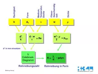
d w = Re w2 2 d* k = pdyn R = d pdyn Fliess-Geschwindigkeit Dichte Medium, Temperatur,Dichte Rauhigkeit Form k dh w d* in mm einsetzen Colebrook- Diagramm Rohrreibungszahl Rohrreibung in Pa/m
Reibungsverluste Die Reibungsverluste einer Rohrstrecke werden berechnet nach:
Einzelwiderstände Richtungsänderungen, Rohreinführungen, Erweiterungen, Einbauten, Armaturen etc. führen zu weiteren Druckverlusten in Rohrleitungen. Diese Druckverluste werden über Widerstandsbeiwerte, so genannte -Werte (Zeta) erfasst.
Äquivalente (gleichwertige) Rohrlängen An Stelle von Zetawerten werden oft auch gleichwertige Rohrlängen angegeben.D. h. x-m Rohr der Dimension y ergeben unter den gleichen Bedingungen, den gleichen Druckverlust wie der entsprechende Widerstandsbeiwert Zeta.