Download
1 / 25
260 likes | 480 Vues
C2: Hydraulic Position Control System. Le Zhang lfz062@mail.usask.ca Rm. 2B60. Objectives. Study the open-loop performance of an electro-hydraulic position control system.

E N D
C2: Hydraulic Position Control System Le Zhang lfz062@mail.usask.ca Rm. 2B60
Objectives • Study the open-loop performance of an electro-hydraulic position control system. • Study the use of Bode plots to create the open and closed loop transfer functions for the electro-hydraulic position control system using experimental data.
Procedure Outline • Review • Study the electro-hydraulic position control system • Frequency Response • Common Bode Plots • Experiment 1: Use function generator to apply sinusoidal input, use output to create Bode Plots and Transfer Functions.
Procedure Outline • Experiment 2: Use signal analyzer to create Bode Plots, using plots create Transfer Functions. • Experiment 3: Use signal analyzer to measure close loop response and compare this to the theoretical response.
Review Outline • Frequency Response • Bode Plots • Experimental System
Review Outline • Frequency Response • Bode Plots • Experimental System
Frequency Response Figure 1: General SISO System Are these the same?
Frequency Response (Con’t) Figure 2: Input-Output response relationship
But what if we want to study the system in the frequency domain?
Frequency Response (Con’t) Laplace Transform: Figure 3: Plant diagram. How do we change from continuous to frequency domain? s → jω Magnitude Frequency Response: Phase Frequency Response:
If the ω changes, the magnitude of output signal (B) and the phase (φ)of output signal will change. • As a consequence, the value of |G(jω)| and ∠G(jω) will change.
Review Outline • Frequency Response • Bode Plots • Experimental System
Bode Plots: Case 1 20 log|K| dB 0 rad/s 0 degrees 0 rad/s
Bode Plots: Case 2 20 -20 dB/decade dB 0 0.1 1 10 rad/s -20 Phase angle 0 -90 degrees
Bode Plots: Case 3 -20 dB/decade 20 log|K| 0 1 rad/sec 0 -90 degrees
Bode Plots: Case 4 -20 dB/decade
Bode Plots: Case 4 -45 -90
Bode Plots: Case 5 Can we simplify? What does ξ really mean? Can we let ξ equal some value to help simplify the equation? ξ = 1
Bode Plots: Case 5 The equation from the last slide may be written as: -90 -180 -40 dB/decade All we need to do is double both of the plots from Case 4
Review Outline • Frequency Response • Bode Plots • Experimental System
Experimental System Function Generator Amplifier Valve Actuator Transducer Recorder
Experimental System (Con’t) Function Generator Amplitude Valve Load Transducer G(s) Recorder
Experiment 1: • Obtain transducer sensitivity, Kv. • Apply sinusoidal input and obtain output. • Create Bode plots from output data. • Obtain open-loop TF. • Predict closed-loop TF.
Experiment 2: • Setup spectrum analyzer. • Obtain data and import to Excel. • Obtain Bode Plots. • Obtain open-loop TF. • Predict closed-loop TF.
Experiment 3: • Close the loop in the system. • Get Bode Plot from the signal analyzer • Draw asymptotes derived from the theoretical model onto the Bode Plot of the experimental results • Compare results