Mathematical Optimization in Process Synthesis and Simulation
This lecture by Dr. Mario Richard Eden from Auburn University covers the fundamentals of mathematical optimization as part of chemical engineering processes. It aims to provide a comprehensive understanding of various optimization problem types, including linear and non-linear programming, integer programming, and their applications in maximizing operational efficiency. The course emphasizes formulating problems using optimization principles and applying software tools like LINGO for practical solutions. Key examples include reactor conversion optimization and cost minimization in plant operations.

Mathematical Optimization in Process Synthesis and Simulation
E N D
Presentation Transcript
Optimization CHEN 4460 – Process Synthesis, Simulation and Optimization Dr. Mario Richard EdenDepartment of Chemical EngineeringAuburn University Lecture No. 8 – Mathematical Optimization October 16, 2012 Contains Material Developed by Dr. Daniel R. Lewin, Technion, Israel
Lecture 10 – Objectives On completion of this part, you should: • Understand the different types of optimization problems and their formulation • Be able to formulate and solve a variety of optimization problems in LINGO
Optimization Basics • What is Optimization? • The purpose of optimization is to maximize (or minimize) the value of a function (called objective function) subject to a number of restrictions (called constraints). • Examples • 1.Maximize reactor conversion • Subject to reactor modeling equations • kinetic equations • limitations on T, P and x
Optimization Basics • Examples (Continued) • 2.Minimize cost of plant • Subject to mass & energy balance equations • equipment modeling equations • environmental, technical and logical constraints
Optimization Basics • Examples (Continued) • 3.Maximize your grade in this course • Subject to extracurricular activities • full-time-job requirements • constant demand by other courses and/or your advisor/boss
Optimization Basics • Formulation of Optimization Problems • min (or max) f(x1,x2,……,xN) • subject to g1(x1,x2,……,xN)≤0 • g2(x1,x2,……,xN)≤0 • gm(x1,x2,……,xN)≤0 • h1(x1,x2,……,xN)=0 • h2(x1,x2,……,xN)=0 • hE(x1,x2,……,xN)=0 Feasibility Any vector (or point) which satisfies all the constraints of the optimization program is called a feasible vector (or a feasible point) The set of all feasible points is called feasibility region or feasibility domain Any optimal solution must lie within the feasibility region! Inequality Constraints Equality Constraints
Optimization Basics • Classification of Optimization Problems • Linear Programs (LP’s) • A mathematical program is linear if • f(x1,x2,……,xN) and gi(x1,x2,……,xN)≤0 are linear in each of their arguments: • f(x1,x2,……,xN) = c1x1 + c2x2 + …. cNxN • gi(x1,x2,……,xN) = ai1x1 + ai2x2 + …. aiNxN • where ci and aij are known constants. Linear Programs (LP’s) can be solved to yield a global optimum. Solver routines can guarantee a truly optimal solution.
Optimization Basics • Classification of Optimization Problems • Non-Linear Programs (NLP’s) • A mathematical program is non-linear if any of the arguments are non-linear. For example: • min 3x + 6y2 • s.t. 5x + xy ≥ 0 • Integer Programming • Optimization programs in which ALL the variables must assume integer values. The most commonly used integer variables are the zero/one binary integer variables. • Integer variables are often used as decision variables, e.g. to choose between two reactor types. Non-Linear Programs (NLP’s) can be solved to yield a local optimum. Solver routines can not always guarantee a globally optimal solution.
Optimization Basics • Classification of Optimization Problems • Mixed Integer Linear Programs (MILP’s) • Linear programs in which SOME of the variables are real and other variables are integers • Can be solved as individual LP’s by fixing the integer variables, thus a global optimum can be identified. • Mixed Integer Non-Linear Programs (MINLP’s) • Non-linear programs in which SOME of the variables are real and other variables are integers • Can be solved as individual NLP’s by fixing the integer variables, but depending on the nature of the NLP’s it may not be possible to find a global optimum.
Optimization Basics • Formulation of Optimization Problems • Step 1 • Determine the quantity to be optimized and express it as a mathematical function (this is your objective function) • Doing so also serves to define variables to be optimized (input variables or optimization variables) • Step 2 • Identify all stipulated requirements, restrictions, and limitations, and express them mathematically. These requirements constitute the constraints • Step 3 • Express any hidden conditions. Such conditions are not stipulated explicitly in the problem, but are apparent from the physical situation, e.g. non-negativity constraints
Optimization Example • Hydrogen Sulfide Scrubbing • Two variable grades of MEA. • First grade consists of 80 weight% MEA and 20% weight water. Its cost is 80 cent/kg. • Second grade consists of 68 weight% MEA and 32 weight% water. Its cost is 60 cent/kg. • It is desired to mix the two grades so as to obtain an MEA solution that contains no more than 25 weight% water. • What is the optimal mixing ratio of the two grades which will minimize the cost of MEA solution (per kg)?
Optimization Example • Hydrogen Sulfide Scrubbing (Cont’d) • Objective function min z = 80x1 + 60x2 • Constraints • Water content limitation 0.20x1 + 0.32x2 ≤ 0.25 • Overall material balance x1 + x2 =1 • Non-negativity x1 ≥ 0 • x2 ≥ 0 Variables (Basis 1 kg solution) x1 Amount of grade 1 (kg) x2 Amount of grade 2 (kg) z Cost of 1 kg solution (cents)
Optimization Example • Hydrogen Sulfide Scrubbing (Cont’d) • Feasibility region • The set of points (x1, x2) satisfying all the constraints, including the non-negativity conditions. • Constraint on water content 0.20x1 + 0.32x2 ≤ 0.25
Optimization Example • Hydrogen Sulfide Scrubbing (Cont’d) • Feasibility region • Non-negativity constraints x1 0 , x2 0
Optimization Example • Hydrogen Sulfide Scrubbing (Cont’d) • Feasibility region • Mass balance constraint x1 + x2 = 1
Optimization Example • Hydrogen Sulfide Scrubbing (Cont’d) • Feasibility region Any optimal solution must lie within the feasibility region!
Optimization Example • Hydrogen Sulfide Scrubbing (Cont’d) • By plotting objective function curves for arbitrary values of z (here 70 and 75) we can evaluate the results: Optimal Point Intersection between x1 + x2 = 1 and 0.20x1 + 0.32x2 = 0.25 In addition 70 < zmin < 75
Optimization Example • Hydrogen Sulfide Scrubbing (Cont’d) • Solving the two equations simultaneously yields the optimum amounts of the two MEA solutions along with the minimum cost of the mixture
Optimization Software • LINGO • Available on computers in Ross 306 • To start entering a new optimization problem type: • Model: • Enter the objective function by typing: • min = ……; or max = ……; • Then enter the constraints. • Each line must end by a semi-colon ; • The final statement in the problem should be “end”
Optimization Software • Resolving MEA Example in LINGO LINGO Input Model: min = 80*x1 + 60*x2; 0.2*x1 + 0.32*x2 < 0.25; x1 + x2 = 1; x1 > 0; x2 > 0; end LINGO Output Rows= 5 Vars= 2 No. integer vars= 0 ( all are linear) Nonzeros= 10 Constraint nonz= 6( 4 are +- 1) Density=0.667 Smallest and largest elements in absolute value= 0.200000 80.0000 No. < : 1 No. =: 1 No. > : 2, Obj=MIN, GUBs <= 2 Single cols= 0 Optimal solution found at step: 0 Objective value: 71.66667 Variable Value Reduced Cost X1 0.5833333 0.0000000E+00 X2 0.4166667 0.0000000E+00 Row Slack or Surplus Dual Price 1 71.66667 1.000000 2 0.0000000E+00 166.6667 3 0.0000000E+00 -113.3333 4 0.5833333 0.0000000E+00 5 0.4166667 0.0000000E+00 Value of objective function: 71.6667 Value of variable x1: 0.5833 Value of variable x2: 0.4167
More Optimization Examples • Lab Experiment • Determine the kinetics of a certain reaction by mixing two species, A and B. The cost of raw materials A and B are 2 and 3 $/kg, respectively. • Let x1 and x2 be the weights of A and B (kg) to be employed in the experiment • The operating cost of the experiment is given by: • OC = 4(x1)2 + 5(x2)2 • The total cost of raw materials for the experiment should be exactly $6. Minimize the operating cost!
More Optimization Examples • Lab Experiment (Cont’d) LINGO Input Model: min = 4*x1^2 + 5*x2^2; 2*x1 + 3*x2 = 6; x1 > 0; x2 > 0; end LINGO Output Rows= 4 Vars= 2 No. integer vars= 0 Nonlinear rows= 1 Nonlinear vars= 2 Nonlinear constraints= 0 Nonzeros= 7 Constraint nonz= 4 Density=0.583 Optimal solution found at step: 4 Objective value: 12.85714 Variable Value Reduced Cost X1 1.071429 0.0000000E+00 X2 1.285714 0.0000000E+00 Row Slack or Surplus Dual Price 1 12.85714 1.000000 2 0.0000000E+00 -4.285715 3 1.071429 0.1939524E-07 4 1.285714 0.0000000E+00 Value of objective function: 12.857 Value of variable x1: 1.071 Value of variable x2: 1.286
More Optimization Examples • Coal Conversion Plant • What are the optimal production rates of gaseous and liquid fuels that maximize the net profit of the plant? x1 ≤ 4 2x2 ≤ 12 3x1 + 2x2 ≤ 18
More Optimization Examples • Coal Conversion Plant (Cont’d) • Objective function max z = 3x1 + 5x2 • Constraints • Pretreatment capacity 3x1 + 2x2 ≤ 18 • Gasification capacity x1 ≤4 • Liquefaction capacity 2x2 ≤12 • Non-negativity x1 ≥ 0 • x2 ≥ 0
More Optimization Examples • Coal Conversion Plant (Cont’d) • Graphical solution • Maximum profit Z = 36 for x1 = 2 and x2 = 6
More Optimization Examples • Coal Conversion Plant (Cont’d) LINGO Input Model: max = 3*x1 + 5*x2; 3*x1 + 2*x2 <= 18; x1 <= 4; 2*x2 <= 12; x1 > 0; x2 > 0; end LINGO Output Rows= 6 Vars= 2 No. integer vars= 0 ( all are linear) Nonzeros= 11 Constraint nonz= 6( 3 are +- 1) Density=0.611 Smallest and largest elements in absolute value= 1.00000 18.0000 No. < : 3 No. =: 0 No. > : 2, Obj=MAX, GUBs <= 2 Single cols= 0 Optimal solution found at step: 1 Objective value: 36.00000 Variable Value Reduced Cost X1 2.000000 0.0000000E+00 X2 6.000000 0.0000000E+00 Row Slack or Surplus Dual Price 1 36.00000 1.000000 2 2.000000 0.0000000E+00 3 0.0000000E+00 1.500000 4 0.0000000E+00 1.000000 5 2.000000 0.0000000E+00 6 6.000000 0.0000000E+00 Value of objective function: 36 Value of variable x1: 2 Value of variable x2: 6
More Optimization Examples • Methanol Delivery • Supply methanol for three Methyl acetate plants located in towns A, B, and C • Daily methanol requirements for each plant: • MeAc Plant location Tons/day • A 6 • B 1 • C 10 • Methanol production plants • MeOH plant 1 2 3 4 • Capacity 7 5 3 2
More Optimization Examples • Methanol Delivery (Cont’d) • Shipping cost (100 $/ton) • Schedule the methanol delivery system to minimize the transportation cost
More Optimization Examples • Methanol Delivery (Cont’d) • We define the transportation loads (tons/day) going from each MeOH plant to each MeAc plant as follows: • Total transportation cost (Z) • Z = 2X1A + X1B + 5X1C + 3X2A + 0X2B + 8X2C + 11X3A + 6X3B + 15X3C + 7X4A + X4B + 9X4C
More Optimization Examples • Methanol Delivery (Cont’d) • Objective function min Z = 2X1A + X1B + 5X1C + 3X2A + 0X2B + 8X2C + 11X3A + 6X3B + 15X3C + 7X4A + X4B + 9X4C • Constraints • Availability/supply X1A + X1B + X1C = 7 • X2A + X2B + X2C = 5 • X3A + X3B + X3C = 3 • X4A + X4B + X4C = 2 • Requirements/demand X1A + X2A + X3A + X4A = 6 • X1B + X2B + X3B + X4B = 1 • X1C + X2C + X3C + X4C = 10
More Optimization Examples • Methanol Delivery (Cont’d) • Constraints • Non-negativity X1A ≥ 0 • X1B ≥ 0 • X1C ≥ 0 • X2A ≥ 0 • X2B ≥ 0 • X2C ≥ 0 • X3A ≥ 0 • X3B ≥ 0 • X3C ≥ 0 • X4A ≥ 0 • X4B ≥ 0 • X4C ≥ 0
Mixed Integer Programs • Use of 0-1 Binary Integer Variables • Commonly used to represent binary choices • Dichotomy modeling
Mixed Integer Programs • The Assignment Problem • Assignment of n people to do m jobs • Each job must be done by exactly one person • Each person can at most do one job • The cost of person jdoing job iis Cij • The problem is to assign the people to the jobs so as to minimize the total cost of completing all the jobs. • We can assign integer variables to describe whether a certain person does a certain job or not
Mixed Integer Programs • The Assignment Problem (Cont’d) • The event of person jdoing job i is designated Xij • The objective function can be written as: • Since exactly one person will do job i, and each person at most can do one job, we get:
Mixed Integer Programs • Plant Layout – An Assignment Problem • Four new reactors R1, R2, R3 and R4 are to be installed in a chemical plant • Four vacant spaces 1, 2, 3 and 4 are available • Cost of assigning reactor i to space j (in $1000) is • Assign reactors to spaces to minimize the total cost
Mixed Integer Programs • Plant Layout (Cont’d) • Let Xij denote the existence (or absence) of reactor i in space j, i.e. if Xij =1 then reactor i exists in space j • Objective function min Z = 15X11 + 11X12 + 13X13 + 15X14 + 13X21 + 12X22 + 12X23 + 17X24 + 14X31 + 15X32 + 10X33 + 14X34 • + 17X41 + 13X42 + 11X43 + 16X44
Mixed Integer Programs • Plant Layout (Cont’d) • Constraints • Each space must be assigned to one and only one reactor • X11 + X12 + X13 + X14 = 1 • X21 + X22 + X23 + X24 = 1 • X31 + X32 + X33 + X34 = 1 • X41 + X42 + X43 + X44 = 1 • Each reactor must be assigned to one and only one space • X11 + X21 + X31 + X41 = 1 • X12 + X22 + X32 + X42 = 1 • X13 + X23 + X33 + X43 = 1 • X14 + X24 + X34 + X44 = 1
Mixed Integer Programs • Plant Layout (Cont’d) • Solve using LINGO • Optimal assignment policy • Reactor R1 in space 2 • Reactor R2 in space 1 • Reactor R3 in space 4 • Reactor R4 in space 3 • Minimum cost • Cost = 11 + 13 + 14 + 11 = $49,000
Lecture 10 – Summary On completion of this part, you should: • Understand the different types of optimization problems and their formulation • Be able to formulate and solve a variety of optimization problems in LINGO
Other Business • Homework • SSLW: 24.1 plus problems posted on class webpage • Due Tuesday October 23 • LINGO software is available on class webpage as zip-file • Next Lecture – October 23 • Heat and Power Integration (SSLW p. 252-261) • Review of Midterm Exam • Thursday October 18 during lab sessions • You will get your tests back to look at during solution review