Optimization
Learn about various types of design optimization methods such as Invent, Trial and Error, and Mathematical. Understand the steps involved, constraints, objective functions, and approaches to achieving optimum design solutions.

Optimization
E N D
Presentation Transcript
Types of Design Optimization • Conceptual: “Invent” several ways of doing something and pick the best. • Trial and Error: Make several different designs and vary the design parameters until an acceptable solution is obtained. Rarely yields the best solution. • Mathematical: Find the minimum mathematically.
Terms in Mathematical Optimization • Objective function – mathematical function which is optimized by changing the values of the design variables. • Design Variables – Those variables which we, as designers, can change. • Constraints – Functions of the design variables which establish limits in individual variables or combinations of design variables.
Steps in the Optimization Process • Identify the quantity or function, U, to be optimized. • Identify the design variables: x1, x2, x3, …,xn. • Identify the constraints if any exist • a. Equalities • b. Inequalities • 4. Adjust the design variables (x’s) until U is optimized and all of the constraints are satisfied.
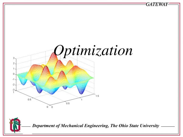
Local and Global Optimum Designs • Objective functions may be unimodal or multimodal. • Unimodal – only one optimum • Multimodal – more than one optimum • Most search schemes are based on the assumption of a unimodal surface. The optimum determined in such cases is called a local optimum design. • The global optimum is the best of all local optimum designs.
The Objective Function, U • Given any feasible set of design variables, it must be possible to evaluate U. Feasible design variables are those which satisfy all of the constraints. • U may be simple or complex. Generally find minimum of the objective function. If the maximum is desired, then find the minimum of the objective function times –1. Max (U) min(-U)
Multimodal Objective Function saddle point local max
Inequality or regional constraints Form: p > 0 Divide the design space into feasible and non-feasible regions. Here the design space is the space defined by the design variables.
Equality or functional constraints Form: For an optimization problem, m < n Often arise from physical properties or laws
Approaches to Mathematical Optimization • Analytical methods – U is a relatively simple, closed-form analytical expression. • Linear Programming methods – U, ’s, and ’s are all linear in x’s. • Nonlinear searches – U, ’s, or ’s are nonlinear and complicated in x’s.
Analytical Methods – One Design Variable There can be no equality constraints on x, since this would make the problem deterministic. Inequality constraints are possible. If U = U(x), the optimum occurs when Must also check boundaries when inequality constraints are involved.
Example – One Design Variable Insulation problem: cost of insulation of thickness x: cost of heat loss during operation: total cost of operation: where a through d are known constants for a minimum cost: so:
Analytical Methods – Several Variables, No Constraints • At an optimum point, • U = U(x1,x2,x3,…,xn) must be nonlinear. • This gives n equations in n unknowns, which can be solved using some nonlinear solution procedure such as Newton’s method. • There are analytical tests for maximum and minimum values involving the Jacobian matrix for U, but it is usually easier to determine this by direct inspection. • Saddle points can be a problem.
Analytical Methods – Several Variables and Equality Constraints • Given: 2. Method 1: • Solve for one of the x’s in the G equations and eliminate that variable in U. • Optimize U with the reduced set of the design variables. • Example:
Method 2 – Lagrange Multipliers 1. Given: • Used when G’s are not used to eliminate variables from U • Procedure: a) Introduce p new variables i such that a new objective function is formed. • Differentiate F as if no constraints are involved.
Method 2 – Lagrange Multipliers cont. • Solve n+p equations in n+p unknowns (x’s and ’s). n equations from p equations from G’s 4. Generally the ’s are of no direct interest if only equality constraints are present.
Example – Lagrange Multipliers Given: 1. Form F: 2. Optimize F:
Example – cont. then and
Linear Programming Given: U(x1,x2,…,xn) is linear i(x1,x2,…,xn) = 0 i = 1,2,…,p are linear I(x1,x2,…,xn) > 0 i = 1,2,…,m are linear • No finite optimum exists unless constraints are present. • The optimum will occur at one of the vertices of the constraint boundaries. • Procedure is to start at one vertex and check vertices in a systematic manner (simplex method).
Linear Programming Example Given: Subject to the following constraints: First find the vertices by combining equations and eliminating vertices that don’t comply to all the constraints:
Linear Programming Objective function contour lines – colored lines i = inequality constraints Fi = vertices
Direct Search Methods – One Design Variable Given: U(x), a<x<b • Vary x to optimize U(x), • Want to minimize number of function evaluations (number of times that U(x) is computed).
Method 1: Exhaustive Search • Divide the range (b-a) into equal segments and compute U at each point. • Pick x for the minimum U. Note that if it is desired to make function evaluations at only n interior points, then the spacing between points, x, will be
Exhaustive search example Given: f() = 72-25+35 Find the minimum over the interval (0,5) using 10 interior points
Method 2: Random Search 1. Objective function is evaluated at numerous randomly selected points between a and b. 2. Choose new interval about the best point. 3. Repeat the procedure until the optimum is established. Points chosen:
Random search example Given: f() = 72-25+35 Find the minimum on the interval (0,5) using 10 interior points
Method 3: Interval Halving Divide the interval into 4 equal sections, resulting in 5 points. Bound the minimum and use the IOU as the new interval. Repeat until the desired accuracy is reached. Determining the IOU: Case 1: if f(2) < f(3), then IOU is from 1 to 3. Case 2: if f(4) < f(3), then IOU is from 3 to 5. Case 3: otherwise IOU is from 2 to 4.
Interval Halving Example Given: f() = 72-25+35 Find the minimum on the interval (0,5) using 9 interior points
Method 4: Golden Section Search 1. Divide the interval such that 2. Evaluate at 4-z2 and 1+z2. • Choose smallest U and reject region beyond large U. • Subdivide new region by the same ratio. 5. Each time there is a function evaluation, the region is reduced to 0.618 times the previous size.
Golden Section Search Example Given: f() = 72-25+35 Find the minimum on the interval (0,5) using 10 interior points
Method 5: Parabolic Search Method 5 – Parabolic search 1. Successively approximate the shape of U as a parabola. 2. Make three function evaluations, pass the parabola through the three points, and find the minimum of the parabola. 3. Keep three best points and repeat the procedure until the optimum is established.
Method 5: Parabolic Search, cont. Need to find the parabola that fits 3 data points. This most easily accomplished by writing the parabola as follows: Now or or
Parabolic Search Example Given: f() = 72-25 + 90 + 50cos(1.4) Find the minimum on the interval (0,5) using 10 interior points
Optimization of Nonlinear Multivariable Systems • Indirect or gradient based methods - must be available. • 2. Direct search methods – vary the x’s to maximize or minimize f directly.
Multivariable Optimization Searches Procedures covered: I. Non-gradient methods: • A. Exhaustive (Grid) search • B. Random search • Box search • Powell’s method II. Gradient methods: • A. Steepest descent procedure • B. Optimum steepest descent procedure • Fletcher-Powell procedure • Powell’s method
Method 1 – Grid Search • Divide the range for each design variable into equal segments and compute U at each point. • 2. Pick x for the minimum U.
Grid Search Example Given: f(x1,x2) = 2sin(1.47 x1) sin(0.34 x2) + sin(x1) sin(1.9 x2) Find the minimum when x1 is allowed to vary from 0.5 to 1.5 and x2 is allowed to vary from 0 to 2.
Method 2 – Random Search 1. Objective function is evaluated at numerous randomly selected points between a and b. 2. Choose new interval about the best point. 3. Repeat the procedure until the optimum is established. Points chosen:
Random Search Example Given: f(x1,x2) = 2sin(1.47 x1) sin(0.34 x2) + sin(x1) sin(1.9 x2) Find the minimum when x1 is allowed to vary from 0.5 to 1.5 and x2 is allowed to vary from 0 to 2.
Method 3 – Box Method Randomly choose 2n points. Identify the worst point. Compute the centroid of the remaining points. Reflect the rejected vertex an amount d through the centroid. If the new vertex violates constraints or is worse than the rejected point, move it closer to the centroid. Repeat until the optimum is found.
Box Method Example Given: f(x1,x2) = 2sin(1.47 x1) sin(0.34 x2) + sin(x1) sin(1.9 x2) Find the minimum when x1 is allowed to vary from 0.5 to 1.5 and x2 is allowed to vary from 0 to 2.
Powell’s method Starting point: Next point: Optimize along each search direction Compute which search direction causes the greatest reduction of the objection function using: Calculate the proposed new search direction: Determine the cost of the objective function at the test point.
Powell’s method, cont. 6. Test to see if the new search direction is good using: Condition 1: Condition 2: If both conditions are true, then is a good search direction and will replace the previous best search direction, xm. 7. Go to step 2 and repeat procedure until the optimum is found.
Example of Powell’s Method Given: f(x1,x2) = 2sin(1.47 x1) sin(0.34 x2) + sin(x1) sin(1.9 x2) Find the minimum when x1 is allowed to vary from 0.5 to 1.5 and x2 is allowed to vary from 0 to 2.