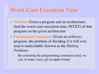
Worst-case Execution Time (WCET) Estimation

1. Worst-case Execution Time (WCET) Estimation Shawn Schaffert

2. Outline • Introduction • WCET problem & analysis • Cinderella before cache modeling • Cinderella with cache modeling • Conclusion

3. Introduction

4. Motivation • Recent growth in embedded systems • Real-time applications have strict requirements • Often assumed by schedulers • Hardware-software partition driven by timing constraints • Impractical to simulate every situation

5. Previous Work & Other Work • General area of program analysis (Nielson, Nielson, & Hankin) • In general, undecidable; equivalent to the halting problem (Puschner, Koza) • Decidable by introducing restrictions (Kligerman, Stoyenko and Puschner, Koza): • No dynamic data structures • No recursion • Bounded loops • Fully associative caches modeling (Theiling, Ferdinand, Wilhelm) • Automatically extracting functional constraints (Gustafsson)

6. WCET Problem

7. Problem Statement • Given: • Program • Processor (and memory system) • Assume: • Uninterrupted execution • Find: • Upper bound on execution time (Tmax) • Lower bound on execution time (Tmin) • Goals: • Try to have tight bounds

8. Key Parts of Analysis • Program path analysis • Sequence of instructions executed in worse (best) case • Micro-architectural modeling • Representation of host processor and memory • Use to compute how much real time is required to execute a sequence of instructions • Interplay between two makes analysis complex

9. Cinderella(Before Cache Modeling)

10. Main Idea • Idea: • Implicitly consider paths (not explicitly) • Divide program into basic blocks • Form problem as a integer linear programming (ILP) problem: • Integer variables: number of executions of each part of program • Linear objective: maximum (minimum) execution time • Linear constraints: structure and function of program • ILP is worst case exponential time, good in practice

11. x1 B1 x3 B3 x2 B2 Divide into basic blocks i = 10; store(i); n = 2*i; store(n); void store(int i) { ... }

12. Objective Function • Bi = basic block i • xi = number of times the block Bi is executed • ci = worst case running time of block Bi • Lower bound computed analogously

13. d1 B1 x1 d4 d2 B3 B2 x2 d3 d5 Program Structural Constraints i = 10; store(i); n = 2*i; store(n); void store(int i) { ... } x1 = d1 = d2 x2 = d2 = d3 d4 = d2 + d3

14. d1 x1 B1 s = k; d2 d8 x2 B2 while (k < 10){ d3 x3 B3 if (ok) d5 B5 d4 j = 0; ok = true; x4 x5 B4 j++; d6 B6 d7 k++; x6 d9 B7 r = j; x7 d10 Program Structural Constraints /* k >=0 */ s = k; while (k < 10){ if (ok) j++; else { j = 0; ok = true; } k++; } r = j;

15. Program Functionality Constraints • Structural constraints abstract functionality away • Program behavior provides more constraints • Loop Bounds

16. Functionality Constraints Constraints check_data() { x1 int i, morecheck, wrongone; x2 morecheck = 1; i = 0; wrongone = -1; x3 while (morecheck) { x4 if (data[i] < 0) { x5 wrongone = i; morecheck = 0; } else x6 if (++i >= 10) x7 morecheck = 0; } x8 if (wrongone >= 0) x9 return 0; else x10 return 1; } x2 x4 x4  10x2 (x5 = 0 & x7 = 1) | (x5 = 1 & x7 = 0) x5 = x9

17. Solving the Constraints • ILP solver requires constraints that are: • equalities • inequalities • conjunctions of the above • Disjunctions  Separate Cases (exponentially many)

18. Micro-architectural Modeling • Simple model to estimate ci’s • Reduce basic blocks to assembly code and use hardware manual to bound each instruction • Does not model cache memory well

19. Cinderella(With Cache Modeling)

20. Cache Modeling • Model direct-mapped instruction cache • Requires: • Modify cost function (cache hit and miss have different costs) • Add linear constraints to describe relationship between cache hits and misses

21. n bits m bits xx..xx 00..00 00…00 … xx..xx 00..00 11…11 xx..xx 00..01 00…00 … xx..xx 00..01 11…11 … … … xx..xx 00..00 00…00 … xx..xx 00..00 11…11 xx..xx 00..01 00…00 … xx..xx 00..01 11…11 … Direct-Mapped Cache Main Memory Cache Memory 2n 2m

22. Basic Idea • Basic blocks assumed to be smaller than entire cache • Subdivide instruction counts (xi) into counts of cache hits (xihit) and misses (ximiss) • Line-block (or l-block) is a contiguous sequence of code within the same basic block that is mapped to the same cache line in the instruction cache • Either all hit or all miss in a l-block

23. B1.1 B1.2 B1.3 B2.1 B2.2 B3.1 B3.2 Example of subdividing basic blocks into line blocks Color Cache Set B1 0 1 2 3 B2 B3

24. ILP Modification • Modified cost function • Cache constraints • Cache conflict graph • User functionality constraints

25. Cache Constraint Examples • No conflicting l-blocks B1 • Two nonconflicting l-blocks are mapped to same cache line B2 B3

26. Cache Conflict Graph • Constructed for every cache set containing two or more conflicting l-blocks • Contains: • start node (represents start of program) • end node (represents end of program) • node Bk.l for every l-block in the cache set • Edge from Bk.l to Bm.n if control can pass between them without passing through any other l-blocks of the same cache set.

27. start p(s,m.n) p(k.l,k.l) p(s,k.l) p(k.l,m.n) Bm.n Bk.l p(m.n,k.l) p(m.n,m.n) p(m.n,e) p(k.l,e) end p(s,e) Cache Conflict Graph Example

28. d1 Cache x1 B1.1 s = k; d2 d8 x2 B2.1 while (k < 10){ d3 x3 B3.1 if (ok) d5 d4 B5.1 x4 B4.1 j = 0; ok = true; x5 j++; d6 d7 x6 B6.1 k++; d9 B7.1 x7 r = j; d10 Cache Constraints Example

29. d1 x1 B1.1 s = k; d2 s d8 x2 B2.1 while (k < 10){ p(s,5.1) d3 p(s,4.1) x3 B3.1 if (ok) p(4.1,4.1) p(4.1,5.1) d5 B4.1 B5.1 d4 B5.1 x4 B4.1 j = 0; ok = true; p(5.1,4.1) x5 j++; p(5.1,5.1) p(4.1,e) d6 p(s,e) d7 p(5.1,e) x6 B6.1 k++; e d9 B7.1 x7 r = j; d10 Cache Constraints Example

30. d1 x1 B1.1 s = k; d2 s d8 x2 B2.1 while (k < 10){ d3 p(s,1.1) x3 B3.1 if (ok) p(1.1,6.1) d5 B1.1 B6.1 d4 B5.1 x4 B4.1 j = 0; ok = true; x5 j++; p(6.1,6.1) p(1.1,e) d6 p(6.1,e) d7 x6 B6.1 k++; e d9 B7.1 x7 r = j; d10 Cache Constraints Example

31. Implementation • Hardware: • Intel QT960 development board • Intel i960KB processor (32 bit RISC processor) at 20MHz • 128KB main memory • 512 byte direct-mapped instruction cache (32 x 16-byte lines) • Software tool Cinderella: • Reads executable code • Constructs control flow graph(CFG) and cache conflict graph(CCG) • Derives structural constraints • Annotates source files • User provides functionality constraints

33. Set of Benchmarks

34. Comparison with actual running times

35. Estimated Cache Misses

36. Function d’s f’s p’s x’s Struct. Cache Funct. ILP branches Time(sec.) check_data 12 0 0 40 25 21 5+5 1+1 0+0 circle 8 1 81 100 24 186 1 1 0 des 174 11 728 560 342 1059 16+16 13+13 171+197 dhry 102 21 503 504 289 777 24x4+26x4 1x8 0x3+2+0+1x2+4 djpeg 296 20 1816 416 613 2568 64 1 87 fdct 8 0 18 34 16 49 2 1 0 fft 27 0 0 80 46 46 11 1 0 line 31 2 264 231 73 450 2 1 3 matcnt 20 4 0 106 59 61 4 1 0 matcnt2 20 2 0 92 49 54 4 1 0 piksrt 12 0 0 42 22 26 4 1 0 sort 15 1 0 58 35 31 6 1 0 sort2 15 0 0 50 30 27 6 1 0 stats 28 13 75 180 99 203 4 1 0 stats2 28 7 41 144 75 158 4 1 0 whetstone 52 3 301 388 108 739 14 1 2 ILP Solver Performance No. of Constraints No. of Variables

37. Conclusions

38. Conclusions and Future Work • Conclusions: • Method to estimate bounds on running time of a program on a given processor • Modeled direct-mapped instruction cache • Uses ILP to consider paths implicitly (not explicitly) • Software tool: cinderella • Future Work • Improving hardware model: data cache memory & register windows • Automatically derive some of the functionality constraints • Adapt cinderella to other embedded platforms (Motorola M68000)