Download
1 / 25
250 likes | 280 Vues
This seminar discusses the design of a static WCET tool, analyzing flow and low-level aspects in processor pipelines for timing computation. It covers flow analysis, global and local low-level analysis, and calculation methods, presenting a comprehensive overview of the WCET process. The seminar delves into timing models, pipeline construction, and tool architecture, emphasizing correctness, efficiency, and broad applicability. The speaker, Sibin Mohan, shares insights on system design, hardware modeling, and the overall methodology involved in determining worst-case execution times.

E N D
Processor Pipelines and Static Worst-Case Execution Time Analysis PhD dissertation by: Jakob Egblom Presented by: Sibin Mohan Sibin Mohan : Systems Group Seminar
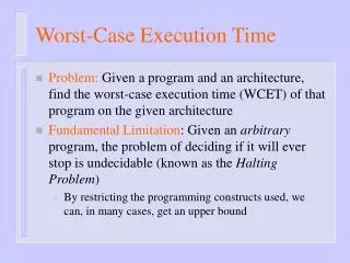
Introduction • Worst-Case Execution Time (WCET) • Timing Analysis • Experimental vs Static Analysis • Processor Pipelines Sibin Mohan : Systems Group Seminar
Pipelines • Various types of pipelines: • Simple scalar pipelines • Scalar pipelines • Superscalar in-order pipelines • VLIW ( Very Long Instruction Word ) • Superscalar out-of-order pipelines Sibin Mohan : Systems Group Seminar
Goals of this work • Design a static WCET tool. • WCET tool must be : • Retargetable • Flexible • Efficient • Broad applicability • Correctness Sibin Mohan : Systems Group Seminar
WCET Overview • Components of WCET Analysis: • Flow Analysis • Global low-level analysis • Local low-level analysis • Calculation Sibin Mohan : Systems Group Seminar
Flow Analysis • Analyze source/object code • Determine possible flow in program • i.e. dynamic behavior of program • Computationally intractable • approximate analysis used. • Three stages : • flow determination • flow representation • preparation for calculation. Sibin Mohan : Systems Group Seminar
Low Level Analysis • Global low-level analysis: • whole program/large parts of it • eg. : cache behaviour/branch prediction • approximate & safe analysis used • can integrate results in two ways: • assign execution time penalty • use as input to local low-level analysis. Sibin Mohan : Systems Group Seminar
Low Level Analysis ( contd. ) • Local low-level analysis : • machine timing of single instructions • egs. : pipeline overlap/memory access • assign execution times to instructions • pipeline overlap -> negative times • overlaps between basic blocks • not necessarily neighbours. Sibin Mohan : Systems Group Seminar
Calculation • Tree-based • Path-based • IPET ( Implicit Path Enumeration ) • Parameterized WCET calculation. Sibin Mohan : Systems Group Seminar
Program Source Manual Annotations i/p data specs Scope Graph Compiler Flow Analysis WCET Calculation Global low-level Analysis Object Code Timing Model Local low-level Analysis WCET Tool Architecture Sibin Mohan : Systems Group Seminar
Local low-level Analysis Scope Graph Object Code Construction of Timing Graph Timing Graph Timing Model CPU Simulator Pipeline Analysis WCET Tool Architecture (contd.) Sibin Mohan : Systems Group Seminar
Timing Model • Abstract representation • Capture exec. time of program • Model timing effects of Pipeline • Compose from smaller parts • Store concrete execution times • Based on timing graph. Sibin Mohan : Systems Group Seminar
Timing Model (contd.) I1…Im – sequence of instructions T( I1…Im ) – time for above instructions Let T(I) = tI – exec time of single instruction To capture pipeline effects, define: Timing effects, Hence, execution time, is: Sibin Mohan : Systems Group Seminar
Timing Model ( contd. ) Sibin Mohan : Systems Group Seminar
Pipeline Model • Single in-order pipeline • n pipeline stages • Each instruction, i, : • sequence of r1i…rni • rji corresponds to execution in stage j • One instruction per stage • All instructions use all stages Sibin Mohan : Systems Group Seminar
Pipeline Model ( contd. ) • Consider execution of I1…Im • For instruction Ii, • let pji – point when Ii enters stage j • and pn+1i is when Ii leaves stage j • This can be modeled as: Sibin Mohan : Systems Group Seminar
Pipeline Model ( contd. ) • Constraints represented as: • Weighted acyclic graph. Sibin Mohan : Systems Group Seminar
Pipeline Model ( contd. ) : Branches and Data Dependences • Branch Instructions : • Data Dependences : Sibin Mohan : Systems Group Seminar
Multiple Parallel Pipelines • Not all instructions use all stages • Each instruction will have: • points corresponding to its entry • points showing actual stages used • The following functions are used : • previ(i,j), nexti(i,j) • prev and next instructions using stage j • prevs(i,j), nexts(i,j) • prev and next stages used by I Sibin Mohan : Systems Group Seminar
Multiple Parallel Pipelines ( contd. ) • Reformulated constraints : • Acyclic Graph : Sibin Mohan : Systems Group Seminar
Prototype • No automatic flow analysis • No global low-level analysis • Two CPU Models : • V580E • ARM 9 • Two calculation modules : • IPET based • Path-based • Cache Analyse implemented • But, not used. • Generates WCET estimates. Sibin Mohan : Systems Group Seminar
Results Sibin Mohan : Systems Group Seminar
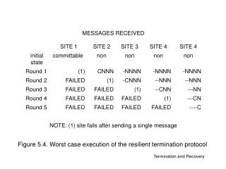
Results ( contd. ) Sibin Mohan : Systems Group Seminar
Conclusions • Contributions : • Formal mathematical model • hardware models • low-level timing modeling scheme • Timing Analysis method • Overall Tool architecture Sibin Mohan : Systems Group Seminar
Thank You ! Further Questions ? Sibin Mohan : Systems Group Seminar