Download
1 / 23
230 likes | 254 Vues
Georg Heygster Institute of Environmental Physics, University of Bremen Arctic GOOS planning meeting Bergen, 12 – 13 September 2006. Sea Ice Remote Concentration charts from AMSR-E 89 GHz data. Overview. Why Remote Sensing of sea ice? Outline of algorithm Operational applications

E N D
Georg HeygsterInstitute of Environmental Physics, University of Bremen Arctic GOOS planning meeting Bergen, 12 – 13 September 2006 Sea Ice Remote Concentration charts from AMSR-E 89 GHz data
Overview Why Remote Sensing of sea ice? Outline of algorithm Operational applications Conclusions and outlook
1. Motivation High resolution sea ice information needed at Low ice concentrations for navigation High ice concentrations for NWP: heat transfer ~ (1-C)
2. ASI (ARTIST Sea Ice) algorithm Svendsen et al. (1987): Use polarization differences near 90 GHz: High for OW Low for all ice types
Daily regional maps Arctic: North West passage Smith Sound Greenland Sea Svalbard Antarctic: Peninsula Ross Sea Scotia Sea Other: Baltic Sea Caspian Sea Sea of Okhotskh Polarstern
Web page – Usage statistics Typical month April 2005: Per day: 2500 hits, 1770 files, 316 pages Total: 2.3 GB, 3400 sites
7. Conclusions and Outlook Daily data available at www.iup.physik.uni-bremen.de Good coincidence with MODIS and Polarstern observations Continued under ESA/EU GMES project Polar View (operations, tbc) EU IP DAMOCLES, Developing Arctic Modelling and Observing Capabilites for Long-term Environment Studies (science) Support offered to GOOS/IPY activities: Provide daily NRT sea ice charts additional maps for user-specified regions time series of historical data Acknowledgements This work was supported by German Research Foundation DFG under grants He 1746/10-1,2,3 EU under project IOMASA (Integrated Observing and Modeling to the Arctic Surface and Atmosphere) EVK3-CT-2002-00067 ESA/EU GMES initiative ICEMON (ESA ESRIN contract 17060/03/I-IW
Backup: RTE for horizontally homogeneous atmosphere surf atm reflected cosmic atm. opacity surf. emissivity
2 fields of progress Using 85/89 GHz data for sea ice concentration AMSR(-E) SSM/I AMSR(-E) Frequency [GHz] Resolution[km x km] Radiometric resolution[K] Frequency [GHz] Resolution [km x km] Radiometric Resolution[K] 6.925 70 x 70 0.3 10.65 50 x 50 0.5 19.35 69 x 43 0.4 18.7 25 x 15 0.5 22.235 60 x 40 0.7 23.8 30 x 18 0.5 37 37 x 29 0.4 36.5 14 x 18 0.5 85.5 15 x 13 0.8 89 6 x 4 1.0 Incidence angle: 53.1° Incidence angle: 55° Swath width: 2400 km Swath width: 1600 km
Bootstrap algorithm Basic Bootstrap Algorithm (BBA, Comiso et al. 2003) Preliminary tie points 19 and 37 GHz: Lower atmosph influence and horizontal resolution (25 km) Condition: C(Bootstrap) < 5% C(ASI) = 0
First Weather Filter: Gradient Ratio (37,19) Gloersen and Cavalieri (1986) for SMMR Illustrated in PR-GR plane Most sensitive to CLW andwind Cuts off C ~ 15 % Condition:GR(37,19) > 0.045 C(ASI) = 0
Second Weather Filter: GR(24,19) Test for high water vapor values Relative Tb change from 19 to 24 GHz Condition:GR(24,19) > 0.04 C(ASI) = 0
Effeciency of Weather Filters Modified 89 GHz Svendsen cloud signature ASI
Cross Validation: Bootstrap BBA (1) ASI – BOOTSTRAP (Baffin Bay), ASI smoothed to 19 GHz, 0% < C < 100 %: mean = -1 +- 4 % cc = 0.99 y = 1.0 x + 0.7
Cross Validation: Bootstrap BBA (2) ASI – BOOTSTRAP (Baffin Bay), ASI smoothed to 19 GHz, 80% < C < 100 %: mean = -1 +- 2 % cc = 0.75 y = 0.6 x + 41.3
Comparison - MODIS black – Land contour green – ASI 15 % White – IED Ice Edge Detection Alg. (Hunewinkel et al. 1998) Kola
ASI algorithm (2) Hybrid algorithm: Modified 89 GHz Svendsen et al. (1987) algorithm for ice covered regions higher resolution Lower frequencies for ice-free ocean less atmospheric effects 3 weather filters: GR(36/19), GR(24/19), Bootstrap algorithm (where C=0) Svendsen et al. 1997 Kaleschke et al. 2001
Modified Svendsen Algorithm Polarization difference near surface... ...and at TOA: a atmospheric Influence, varies with C, approach Determine from known for C=0 and 1 (tie points P0 , P1), dC/dP(C=0 and 1) and ratio C ice concentration PI polarization difference of ice PWpolarization difference of water (Svendsen 1987)