The Virtual Test Facility

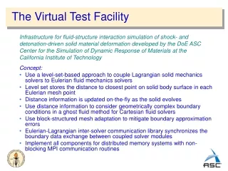
1. The Virtual Test Facility Infrastructure for fluid-structure interaction simulation of shock- and detonation-driven solid material deformation developed by the DoE ASC Center for the Simulation of Dynamic Response of Materials at the California Institute of Technology Concept: • Use a level-set-based approach to couple Lagrangian solid mechanics solvers to Eulerian fluid mechanics solvers • Level set stores the distance to closest point on solid body surface in each Eulerian mesh point • Distance information is updated on-the-fly as the solid evolves • Use distance information to consider geometrically complex boundary conditions in a ghost fluid method for Cartesian fluid solvers • Use block-structured mesh adaptation to mitigate boundary approximation errors • Eulerian-Lagrangian inter-solver communication library synchronizes the boundary data exchange between coupled solver modules • Implement all components for distributed memory systems with non-blocking MPI communication routines

2. VTF software modules • Parallel 3-D Eulerian AMR framework Amroc by R. Deiterding with a suite of shock-capturing finite volume fluid solvers • Hydrid WENO-TCD method by D. Hill and C. Pantano with LES model for compressible flows by D. Pullin • Clawpack version with extended higher-order capabilities and large number of Riemann solver • Complex boundary handling through level-set functions (e.g. through CPT) fully incorporated into AMR algorithm • Parallel 3-D Lagrangian finite element solid mechanics solvers • Thin-shell solver with fracture and fragmentation capability by F. Cirak • Shock-capturing volume solver Adlib by R. Radovitzky et. al • Interface to LS-Dyna • Eulerian-Lagrangian inter-solver coupling (ELC) module by S. Mauch • Closest-point-transform (CPT) algorithm for efficient level set evaluation for triangulated surface meshes by S. Mauch Current portion of source code size of VTF software components

3. VTF source code • Language: object-oriented C++ with components in C, F77, F90. Size ~12MB • ~430,000 lines of source code (ANSI) • autoconf / automake environment with support for typical parallel high-performance systems • Webpage: http://www.cacr.caltech.edu/asc • Installation, configuration, examples • Scientific and technical papers • Archival of key simulation and experimental results • Source code documentation • Downloadable software with example simulations (before end ’06)

4. Fluid-structure coupling in the current VTF • Current software tailored to high-speed events! • Couple compressible Euler equations to Lagrangian structure mechanics • Compatibility conditions between inviscid fluid and solid at a slip interface • Continuity of normal velocity: uSn = uFn • Continuity of normal stresses: Snn = -pF • No shear stresses: Sn = Sn = 0 • Time-splitting approach for coupling • Fluid: • Treat evolving solid surface with moving wall boundary conditions in fluid • Use solid surface mesh to calculate fluid level set through CPT algorithm • Use nearest velocity values uS on surface facets to impose uFn in fluid • Solid: • Use interpolated hydro-pressure pF to prescribe Snn on boundary facets • Ad-hoc separation in dedicated fluid and solid processors

5. Algorithmic approach for coupling Fluid processors Solid processors Update boundary Efficient non-blocking boundary synchronization exchange (ELC) Send boundary location and velocity Receive boundary from solid server Compute level set via CPT and populate ghost fluid cells according to actual stage in AMR algorithm Receive boundary pressures from fluid server AMR Fluid solve Update boundary pressures using interpolation Apply pressure boundary conditions at solid boundaries Do N Sub- Itera- tions Send boundary pressures Solid solve Compute next possible time step Compute next time step Compute stable time step multiplied by N

6. Fluid-structure coupling example • 3d simulation of plastic deformation of thin copper plate attached to the end of a pipe due to water hammer • Strong over-pressure wave in water is induced by rapid piston motion at end of tube • Simulation by R. Deiterding, F. Cirak. Experiment by V.S. Deshpande et al. (U Cambridge) • Motivation: • Validate fluid-structure methodology for plastic deformation Comparison of plate at end of simulation and experiment (middle and right). Left: Fluid-structure interaction ~770s after the wave impact. High fluid pressure (shown in upper half of plane) forces the plate outwards. Color of plate and lower half of plane shows the normal velocity.

7. Water hammer simulation details Fluid • Pressure wave generated by solving equation of motion for piston during fluid-structure simulation, Initial peak pressure: p0=34MPa • Water shock tube of 1.3m length, 64mm diameter • Modeling of water with stiffened equation of state with =7.415, pinf=296.2 MPa • Multi-dimensional 2nd order upwind finite volume scheme, negative pressures from cavitation avoided by energy correction • AMR base level: 350x20x20, 2 additional levels, refinement factor 2,2 • Approx. 1.2.106 cells used in fluid on average instead of 9.106 (uniform) Solid • Copper plate of 0.25mm, J2 plasticity model with hardening, rate sensitivity, and thermal softening • Solid mesh: 4675 nodes, 8896 elements • 8 nodes 3.4 GHz Intel Xeon dual processor, Gigabit ethernet network, ca. 130h CPU to t=1000 s Levels of fluid mesh refinement (gray) ~197s after wave impact onto plate.

8. Detonation-driven fluid-structure interaction • Motivation: Validate VTF for complex fluid-structure interaction problem of detonation-driven rupture of thin aluminum tubes • Interaction of detonation, ductile deformation, fracture • Experiments by T. Chao, J. C. Krok, J. Karnesky, F. Pintgen, J.E. Shepherd • Simulations by R. Deiterding, F. Cirak • Modeling of ethylene-oxygen detonation with constant volume burn detonation model • Thin boundary structures or lower-dimensional shells require “thickening” to apply ghost fluid method • Unsigned distance level set function j • Treat cells with 0<j<d as ghost fluid cells (indicated by green dots) • Leaving j unmodified ensures correctness of rj • Refinement criterion based on j ensures reliable mesh adaptation • Use face normal in shell element to evaluate in  p= pu– pl

9. Fluid solver validation – v venting event • C2 H4+3 O2 CJ detonation for p0=100kPa expands into the open through fixed slot • External transducers to pick up venting pressure • Motivation: • Validate 3D fluid solver with detonation model Simulation • 2nd order upwind finite volume scheme, dimensional splitting • AMR base level: 108x114x242, 4 additional levels, refinement factor 2,2,2,2 • Approx. 6.106 cells used in fluid on average instead of 12.2.109 (uniform) • Tube and detonation fully refined • No refinement for z<0 (to approximate Taylor wave) • No maximal refinement for x>0.1125m, y>0.1125m, z<0.37m, z>0.52m • Thickening of 2d mesh: 0.445mm on both sides additional to real thickness of both sides 0.445mm • Solid mesh: 28279 nodes, 56562 elements • 16 nodes 2.2 GHz AMD Opteron quad processor, Infiniband network, ca. 3300h CPU to t=3000 s

10. Venting event – computational results Comparison of simulated and experimental results at t=0 s Comparison of simulated and experimental results at t=30 s Comparison of simulated and experimental results at t=60 s Comparison of simulated and experimental results at t=90 s

11. Fluid-structure interaction validation – tube with flaps • C2 H4+3 O2 CJ detonation for p0=100kPa drives plastic opening of pre-cut flaps • Motivation: • Validate fluid-structure interaction method • Validate material model in plastic regime Fluid • Constant volume burn model • AMR base level: 104x80x242, 3 additional levels, factors 2,2,4 • Approx. 4.107 cells instead of 7.9.109 cells (uniform) • Tube and detonation fully refined • Thickening of 2d mesh: 0.81mm on both sides (real thickness on both sides 0.445mm) Solid • Aluminum, J2 plasticity with hardening, rate sensitivity, and thermal softening • Mesh: 8577 nodes, 17056 elements • 16+2 nodes 2.2 GHz AMD Opteron quad processor, PCI-X 4x Infiniband network • Ca. 4320h CPU to t=450 s

12. Tube with flaps – computational results Simulated results at t=2 s Simulated results at t=32 s Simulated results at t=62 s Simulated results at t=92 s Simulated results at t=152 s Simulated results at t=212 s Experimental results at t=0 s Experimental results at t=30 s Experimental results at t=60 s Experimental results at t=90 s Experimental results at t=150 s Experimental results at t=210 s

13. Tube with flaps – computational results Fluid density and displacement in y-direction in solid

14. Tube with flaps – fluid mesh adaptation Schlieren plot of fluid density on refinement levels

15. Detonation propagation 41 mm Coupled fracture simulation • C2 H4+3 O2 CJ detonation for p0=180kPa drives tube fracture • Motivation: Full configuration Fluid • Constant volume burn model • 40x40x725 cells unigrid Solid • Aluminum, J2 plasticity with hardening, rate sensitivity, and thermal softening • Material model for cohesive interface: Linearly decreasing envelope • Mesh: 206208 nodes • 27 nodes Lawrence Livermore ASC Linux Cluster with 33 shell and 21 fluid processors • Ca. 972h CPU 45.7 cm Torque 136 Nm Initial crack (6.32 cm)

16. Coupled fracture simulation