Title
Explore applications of inverse and receptor modeling for constraining isoprene emissions using satellite observations. Learn about tropospheric O3 and VOCs, and the challenges in estimating O3 levels. Discover the importance of Global Ozone Monitoring Experiment (GOME) data in understanding atmospheric chemistry.

Title
E N D
Presentation Transcript
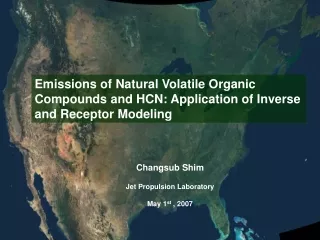
Title Emissions of Natural Volatile Organic Compounds and HCN: Application of Inverse and Receptor Modeling Subtitle Changsub Shim Jet Propulsion Laboratory May 1st , 2007
Outlines 1. Inverse Modeling: Constraining global biogenic isoprene emissions with GOME HCHO columns. 2. Receptor modeling: Source characteristics of OVOCs and HCN. 3. Current TES O3 and CO results: O3-CO correlations to capture pollution outflows.
I. Application of Inverse Modeling: Constraining Global Isoprene Emissions with GOME HCHO Column Measurements Changsub Shim, Yuhang Wang, Yunsoo Choi Georgia Institute of Technology Paul Palmer Leeds University, UK Kelly Chance Harvard-Smithsonian Center for Astrophysics • Shim, C., Y. Wang, Y. Choi, P. Palmer, D. Abbot, and K. Chance, "Constraining global isoprene emissions with Global Ozone Monitoring Experiment (GOME) formaldehyde column measurements," J. Geophys. Res., 110, D24301, doi:10.1029/2004JD005629, 2005.
Tropospheric O3 & VOCs stratosphere Troposphere
Tropospheric O3 • O3 is a precursor of OH, the most important oxidant in the troposphere. • O3 also indirectly determine the lifetime of greenhouse gases. • Environmental Consequences: Surface O3. • There are diverse sources of O3. • * Secondary production in the troposphere: NOx and VOCs • * Transport from the stratosphere • Difficult to estimate the exact amount & distributions of tropospheric O3 and OH
Objectives • Improve the estimates of terrestrial biogenic isoprene emissions: constraining biogenic isoprene emissions with satellite-observed HCHO columns (Inverse modeling & Global CTM).
Global Isoprene (C5H8) • A major natural VOC in the troposphere (e.g., GEIA ~500 Tg/yr; ~ 40% of total VOCs) effect on tropospheric OH & O3 contribution to SOAs • Source: emitted from terrestrial biosphere difficult to measure global emissions (highly uncertain !) • Emissions are dependent upon light intensity, temperature & leaf area, vegetation type, etc. • Main Sink: photolysis by OH Produce HCHO via OH oxidation • Very short lifetime (< hour)
HCHO for constraining Global Isoprene • A high-yield oxidation product of isoprene, other VOCs & Methane. • HCHO atmospheric columns have been measured by a satellite instrument (GOME) at 337 ~ 356 nm. • It also has a short lifetime (order of hours). • HCHO above its background level by CH4-oxidation is a good proxy for isoprene by remote sensing. (Chance et al., 2000; Palmer et al., 2003)
HCHO Space Measurements (GOME) • GOME instrument is on board the ERS-2 satellite. • GOME moves in descending node passing equator at 10:30 AM L.T. in a sun-synchronous orbit. • Nadir-view mode, 40 x 320 km2 resolution, ~3day for global coverage. • GOME measures solar backscattered radiance (UV regions (337 – 356 nm) for HCHO measurements) • Vertical Column Density (VCD) is obtained after retrieval processes including signal fitting, AMF calculations, corrections of device error (e.g., diffusive plate) overall uncertainty is 50 – 70%.
HCHO Space Measurements (GOME) Annual Average From Sep 1996 to Aug 1997
Inverse Modeling • Make a statistical inference of physical parameters (e.g., isoprene base emissions) derived from measurements (e.g. GOME HCHO columns). Physical parameter(“causes”) “Effects” Forward model (ex. CTM) Prediction (Model HCHO column) e.g., a priori Isoprene base emissions, etc. Measurements (ex. GOME HCHO) e.g., a posteriori Isoprene base emissions Inverse model a priori physical parameters e.g., a priori isoprene base emissions
Inverse Modeling y = Kx + e • Bayesian Least Squares (Rodgers, 2000) y : observations (GOME HCHO) x : defined source parameters: GEOS-Chem K : Jacobian matrix (sensitivity of x to y :GEOS-Chem) e : error term We can estimate a posteriori source parameters (x’: “Best Guess”) by calculating Maximum likelihood P(x|y) . A posteriori parameter A posteriori A posteriori error observation A priori
Inverse Modeling • Forward Modeling (GEOS-Chem) • Global CTM • - 3D meteorological fields • - 4º x 5º horizontal resolutions 26 vertical layers • - Ox-NOx-VOC chemical mechanism • - Isoprene emission scheme (Guenther et al., 1995; Wang et • al., 1998) a priori annual isoprene emission: ~ 400 Tg/yr • - Simulated HCHO columns are sampled along the GOME • tracks at the observation time (10 – 11 A.M. LT).
Inverse Modeling Inversion parameters (10 isoprene-emitting vegetation groups + 2) for HCHO V1: Tropical rain forest V2: Grass lands V3: Savanna V4: Tropical seasonal forest V5: Mixed deciduous V6: Farm land & paddy rice V7: Dry evergreen V8: Regrowing wood V9: Drought deciduous V10: Other biogenic source Biomass burning emission Industrial emission Large uncertainties: isoprene emissions from each ecosystem: at least 300%
Inverse Modeling • Regions for Inversions • 8 continental regions are determined by high Signal-to-noise ratio in GOME HCHO measurements (slant column/ fitting error > 4) • Account for ~65% of global a priori isoprene emissions • Each region is inverted separately • Inversion for monthly average HCHO during growing season • Annual a posteriori isoprene emissions are obtained by GEOS-Chem simulation with a posteriori isoprene base emissions over extended rectangular regions.
Regional & Monthly Variations R = 0.84 Bias = -14% GOME HCHO A Priori A posteriori (linear) A posteriori (nonlinear) R = 0.56 Bias = -46%
Discrepancy over the Northern Equatorial Africa Different seasonal HCHO cycle
The Impact of a posteriori Isoprene Emissions Higher a posteriori isoprene emissions reduces the global mean OH concentration by 11%. Tropical upper tropospheric reduction is significant. The corresponding CH3CCl3 lifetime is increased from 5.2 to 5.7 years (e.g., 5.99 years Prinn et al., 2001.)
Findings from Inverse Modeling (Summary) • Global a posteriori isoprene annual emission is higher by 50% to 566 Tg/yr (a priori : 375 Tg/yr). The a posteriori global isoprene annual emissions are generally higher at mid latitudes and lower in the tropics when compared to the GEIA inventory • The a posteriori results suggest higher isoprene base emissions for agricultural land and tropical rain forest and lower isoprene base emissions for dry evergreen • The a posteriori uncertainties of emissions, although greatly reduced, are still high (~90%) reflecting the relatively large uncertainties in GOME retrievals. • There is a significant discrepancy between the seasonality of GOME measured and GEOS-Chem simulated HCHO columns over the northern equatorial Africa. We attribute this problem to the incorrect seasonal cycle in surface temperature in GEOS-STRAT. As a result, isoprene emissions over the region are overestimated.
II. Application of Receptor Modeling : Source Characteristics of Oxygenated Volatile Organic Compounds& Hydrogen Cyanide Changsub Shim and Yuhang Wang Georgia Institute of Technology Hanwant Singh NASA Donald Blake Univ. of California, Irvine Alex Guenther UCAR • Shim, C., Y. Wang, H. B. Singh, D. R. Blake, and A. B. Guenther, Source characteristics of oxygenated volatile organic compounds and hydrogen cyanide, submitted to J. Geophys. Res. 2006.
Receptor Modeling • Emission based vs. Receptor model 1) Emission based model: Use various current knowledge (e.g., sources types, emission rates, transport, chemistry and deposition. etc) to predict air quality (e.g., CTM). 2) Receptor model: Use measured ambient air samples with multivariate statistical method to identify source types and estimate those contributions to measured species (e.g., PCA, CMB, PMF).
Receptor Modeling Positive Matrix Factorization (PMF) Factor Analysis identifying factors based on the covariance btw tracers (e.g., PCA). Includes advanced schemes for optimized solutions and providing tracer’s compositions and reciprocal time series patterns of factors. - It can include the missing values and below detection limits - Treatments of outliers - Positive factor profiles Easier physical interpretation - Statistically optimized results obtained robust results. Advantage over emission based model When CTM has large & complex uncertainties in emissions, chemistry, and transport.
PMF Methods EV (Explained Variation) EV is a relative fraction of each tracer in each factor! Let X is an (n x p) measurement matrix (n: sample observations , p : chemical species). • If we set up the number of factors, k, PMF decomposes X into, X= GF + E Where G (n x k) represents factor scores and F (k x p) represents chemical compositions of factor (factor profile). Or Where i = 1,…,n (# of data) j = 1,…,p (# of tracers) k =1,…,l (# of factors)
PMF methods • Limitations Statistical uncertainties. Difficult to quantify primary emissions for tracers with large 2nd productions. Effect of transport and mixing: difficult to measure the correct contributions. We only choose the results that physically make sense for the study. Additional investigations would be useful (e.g., back trajectories, factor correlations).
Objectives • Investigate source characteristics & contributions to important OVOCs (acetone, methanol, acetaldehyde, etc) and HCN (Receptor modeling)
Measurements Tracer selection from TRACE-P & PEM-Tropics B * Only coincident measurements are selected
Measurements TRACE-P March – April 2001 Asian outflow Latitudes: 15 – 45ºN Longitudes: 114ºE – 124ºW PEM-Tropics B March – April 1999 Tropical Pacific Latitudes: 36ºS – 35ºN Longitudes: 162ºE – 107ºW
Factor Characteristics of TRACE-P CH3OH CH3CN CH3Cl Acetone HCN HCN CO C2H2 i-Pentane CO CHBr3 C2H6 CH3CHO
Factor characteristics of TRACE-P Cyanogenesis (Fall et al., 2003) • Previously, the majority of HCN source is known to be biomass burning. • CN is toxic and various plants (e.g., food crops, clovers, eucalyptus) emit HCN via metabolic processes for self-defense against herbivores. • 41% of HCN (72 pptv) and 40% of acetone (215 pptv) variabilities are possibly associated with terrestrial biogenic emissions • Fairly stable feature is shown in PMF analysis • Does HCN have a large biogenic origin? Acetone + HCN Glucosidase Linamarin Acetone Cyanohydrin Plant Cell H+ Hydroxynitrile lyase H3C CN H3C CN H3C ß-glucosidase =O + HCN H3C O-ß-glucouse H3C O-H H3C Linamarin Acetone Cyanohydrin Fall, R. (2003), Abundant oxygenates in the atmosphere: A biochemical perspective, Chem. Rev., 103, 4,941 – 4, 951.
Factor Characteristics of TRACE-P CH3OH CH3CN CH3Cl Acetone HCN HCN CO i-Pentane C2H2 CO CHBr3 C2H6 CH3CHO
Factor Characteristics of PEM-Tropics B CH3Cl CH3OH CH3CHO CO acetone C2H2 C2H6 CHBr3
Comparison with Global Estimates Global estimates are compiled from Heikes et al. (2002), Li et al. (2003), Singh et al. (2004), and Jacob et al. (2002, 2005). * Others denotes secondary productions in global estimates and error fraction in PMF. • The majority of methanol is from biogenic sources. • The biogenic acetone is a major primary source and photochemical productions are also significant, which is not captured in PMF. • Short life time of acetaldehyde makes secondary productions important and it is hard to quantify the contributions. Large regional variation of oceanic source is shown. • Terrestrial biogenic contributions are likely to be much larger than previous estimation, which may imply the significant influence of cyanogenic productions in plants.
Findings from the PMF study (Summary) • The terrestrial biogenic contribution is a majority of CH3OH sources and is fairly consistent with the global biogenic emission estimates. • The terrestrial biogenic contribution of HCN in TRACE-P (41%) is substantially higher than the global emission estimates (0 – 18%), which suggests that the cyanogenesis in plants from widely dispersed regions is likely to be a major source of HCN over Asia in addition to biomass burning. • The biogenic contribution to CH3COCH3 variability is comparable with the global emission estimates (20 – 40% and 27 – 53%, respectively). However, there are much larger CH3COCH3 industry/urban and biomass burning contributions (8 – 30% and 19 – 55%, respectively) in this study than previous global estimates (1 – 4% and 4 – 10%, respectively), reflecting the importance of secondary productions. We do not find large oceanic contributions to CH3COCH3. • Considering its relatively short lifetime, the large contributions to CH3CHO variability from industry/urban 1 (32%) for TRACE-P and from biomass burning (64%) for PEM-Tropics B imply that secondary production from combustion/industrial VOCs is likely an important sources. The oceanic CH3CHO contribution (10 – 32%) shows the regional dependence and it is lower than previous global emission estimates (63%).
Characterizing Megacity Pollution and Its Regional Impact with TES Measurements Changsub Shim, Qinbin Li, Ming Luo, Susan Kulawik, Helen Worden, and Annmarie Eldering The Jet Propulsion Laboratory California Institute of Technology Pasadena, California 3rd GEOS-Chem User’s Meeting DC8 photo of Mexico City by Cameron McNaughton, University of Hawaii , Feb 2006
Mapping pollution outflow using O3-CO correlation • The observed O3-CO relationship has been used to characterize continental pollution outflow [Fisherman and Seiler, 1983; Chameides et al., 1987; Parrish et al., 1993, etc.]. Positive O3-CO correlations and ∆O3/∆CO indicate photochemical O3 productions. • Tropospheric Emission Spectrometer (TES) aboard the Aura satellite provides concurrent O3 and CO retrievals andvertical profiles. TES O3-CO correlation (at 618 hPa) has been used to map global continental pollution outflow [Zhang et al., 2006]. Parrish et al., JGR1998 O3-CO correlations in surface and aircraft data have been used to test understanding of ozone production but the data are sparse.
O3-CO correlations Zhang, L. et al., 2006
Objectives • Can we characterize megacity pollution and its regional impactwith TES tropospehric ozone and CO retrievals? • We analyzed TES O3 and CO data over the Mexico City Metropolitan Area (MCMA) and Southern U.S. (15-30°N and 90 - 105°W) during the MILAGRO/INTEX-B campaign (March 2006). • We first compared TES O3 and CO retrievals with those from airborne measurements (C130 & DC8 flights) during this campaign. • The comparisons of O3-CO correlation between airborne measurements, TES retrievals, and GEOS-Chem model were then used to evaluate the TES capability to characterize urban outflow on a regional scale.
Mexico City Metropolitan Area (MCMA) (19°N, 99°W) • 2nd largest metropolitan area in the world (~20 million inhabitants) within area of ~1,500 km2. • MCMA is surrounded by mountains and thermal inversions often trap pollution within the basin. • The elevation (~750 hPa) is about 2.2 km above mean sea level. Lower pO2 makes combustion ineffective, which enhances emissions of CO, VOCs, and O3. • Motor vehicular exhaustion is a very important source of air pollution (3 million aged vehicles).
In-situ measurements during MILAGRO/INTEXB (C130 and DC8 ) • NSF C-130 for MILAGRO covers (16 – 25°N and 93 – 101°W) in Mar 2006 (red). • NASA DC-8 for INTEX-B covers (15 – 35°N and 90 - 103°W) (blue). • ~6,000 coincident measurements of O3 and CO from the two aircrafts (5-min merge).
TES retrievals • On-board the Aura satellite launched in July 2004 to provide simutaneous 3-D mapping of tropospheric O3, CO, HDO and CH4, amongother species globally. • The Aura satellite moves in polar sun-synchronous orbit at 705 km height in the ascending node passing equator at 0145 and 1345 LT (16 days for global coverage). • TES has a spatial resolution of 5 x 8 km in nadir-viewing mode. • TES has the standard observations (“global surveys”: 108 km apart along the track) and the special observations (“step and stares”) with denser nadir coverage (45 km apart). • 11 step and stares and 5 global surveys were used in this study for the MILAGRO/INTEX-B periods. • Version 2 data (V002, F03_03) with better quality flags.
TES orbital tracks over MCMA during MILAGRO/INTEX-B Typical TES O3 and CO Averaging Kernel Step and stare Mar 12th , 2006.
GEOS-Chem simulations • GEOS-4 met fields (2x2.5° with 30 layers) from NASA GMAO. • Standard full chemistry simulations (O3-NOx-VOC) [version 7- 04 -10]. • Monthly biomass burning emission inventory [Duncan et al., 2003]. • Fossil fuel emission inventory: EDGAR inventory scaled for time and the model grid [Benkovitz et al., 1996; Bey et al., 2001]. EPA/NEI 99 and BRAVO inventories [U.S. EPA, 2004; Kuhns et al., 2005] are used for U.S. and Mexican fossil fuel emissions respectively. • Lightning NOx emissions with parameterization based upon cloud top height and regionally scaled to OTD/LIS observations. • Biogenic emissions: MEGAN inventory [Guenther et al., 2006]. • 3-hour O3 and CO model results were sampled along TES orbits. • For comparison with TES retrievals, local TES averaging kernels were applied to GEOS-Chem vertical profiles [Zhang et al, 2006].
Observed (in-situ) vertical distributions of O3, CO, and NOx (Mar. 2006) O3 CO NOx Altitude of MCMA ! • MCMA pollution outflow concentrated at 600-800 hPa. • TES has large sensitivity to 600 – 800 hPa pressure levels. • TES data are ideal for analyzing the MCMA outflows!
Comparisons of O3 over the MCMA (Mar. 2006) There is considerable O3 enhancement in the in situ data at 600 – 800 hPa over MCMA. The enhancement is not apparent in TES data nor GEOS-Chem results.
Comparisons of CO over the MCMA (Mar. 2006) The CO enhancement in aircraft data over MCMA at 600 – 800 hPa is not apparent in TES retrieval nor GEOS-Chem results. Why?
C130+DC8 GC raw TES (co-located) TES (all) Time series (daily) comparisons over the MCMA (C130 & DC8 coverage gridded in 2 x 2.5°) between 600 – 800 hPa • TES orbit did not cover the MCMA for the days of three high pollution events (Mar. 9th, 22th, and 29th.). • But the TES data generally show good agreements with aircraft measurements. • The GEOS-Chem model underestimates both O3 and CO by ~29% and ~45% respectively (at 600 – 800 hPa).