Classification: Linear Models

1. Classification: Linear Models Prof. NavneetGoyal CS & IS BITS, Pilani

2. Classification • By now, you are well aware of the classification problem • Assign an input vector x to one of the K discrete disjoint classes, Ck • Overlapping classes: Multi-label classification – has many applications • Classifying news articles • Classifying research articles • Medical diagnosis • Input space is partitioned into decision regions whose boundaries are called decision boundaries or decision surfaces • Linear models for classification • Decision surfaces are linear fns. of the input vector x • (D−1) dim. hyperplane within D-dim. input space • Data sets whose classes can be separated exactly by linear decision surfaces are said to be linearly separable

3. Classification • In regression, the target variable t was simply the vector of real nos. whose values we wish to predict • In classification, there are various ways of using t to represent class labels • Binary class representation is most convenient for probabilistic models • Two class: t ∈ {0, 1}, t = 1 represents C1, t = 0 rep class C2 • Interpret value of t as the probability that class is C1 • Probabilities taking only extreme values of 0 and 1 • For K > 2 - Use a 1-of-K coding scheme. • Eg. K = 5, pattern of class 2 has target vector t = (0, 1, 0, 0, 0)T • Value of tk interpreted as probability of class Ck

4. Classification • Three different approaches: • Simplest: construct a discrimination fn that directly assigns each vector x to a specific class • Model the conditional probability p(Ck|x) in an inference stage, and then use this distribution to make optimal decisions • What are the benefits of separating inference & decision? • Two ways of doing this: • Option 1: Find p(x|Ck) and prior class probabilities p(Ck) and apply Bayes’ theorem • Option 2: Find joint prob. distribution p(x,Ck) directly and then normalize to obtain the posterior probabilities

5. Classification Three different approaches • Discriminative Approach • Direct mapping form inputs x to one of the classes • No direct attempt to model either the class conditional or posterior class probabilities • Examples include Perceptrons, Discriminant functions, SVMs • Regression Approach • Class-conditional Approach

6. Classification Three different approaches • Discriminative Approach • Regression Approach • Posterior class probabilities p(Ck|x) are modeled explicitely • For prediction, the max of these probs. (possibly weighted by a cost fn.) is chosen • Logistic regression • Decision tress • DISCRIMINATIVE – IF TREE ONLY PROVIDES THE PREDICTED CLASS AT EACH LEAF • REGRESSION – IF IN ADDITION THE TREEE PROVIDES POSTERIOR CLASS PROB. DISTR. AT EACH LEAF • Class-conditional Approach

7. Classification Three different approaches • Discriminative Approach • Regression Approach • Class-conditional Approach • Class conditional distributions p(x|Ck, θk) are modeleld explicitly and along with estimates of p(ck) are inverted visBayes’ rule to arrive at p(Ck|x) for each class Ck, a max. is picked • θk are unknown parameters governing the ch. Of class Ck.

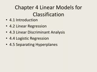
8. Discriminant Functions • Definition • Linear discriminant functions • 2-class problem & extension to K>2 classes • Methods to learn parameters • Least squares classification • Fisher’s linear discriminant • Perceptrons

9. Discriminant Functions • Definition: A discriminant is a fn. that takes an input vector x and assigns it to one of K classes • Linear discriminant functions: Decision surfaces are hyperplanes • Searches for the linear combination of the variables that best separates the classes • Discriminative approach since it does not explicitly estimate either the posterior probabilities of classes or the class-conditional distributions

10. Discriminant Functions Figure: In red, the first class. In green, the second one. In blue, the analytic decision boundary. The train examples are 0, the test ones + (taken form plearn.berlios.de) mblondel.org

11. Discriminant Functions springerimages.com http://cnx.org/content/m11531/latest/

12. Discriminant Functions Linear Discriminant Function with K=2 Figure taken from Bishop CM’s book – Pattern recognition & ML, Springer 2006.

13. Discriminant Functions 2 –class Linear Discriminant Function for K=3 (2 binary DFs) 1 vs. rest approach Figure taken from Bishop CM’s book – Pattern recognition & ML, Springer 2006.

14. Discriminant Functions 2 –class Linear Discriminant Function for K>2 (K*(K-1)/2) binary DFs) 1 vs. 1 approach Figure taken from Bishop CM’s book – Pattern recognition & ML, Springer 2006.

15. Discriminant Functions • Consider a single K-class DF comprising K linear fns. of the form: • Assign a point x to class Ck if • Decision boundary between Ck & Cj is therefore given by and hence corresponds to a (D-1) dimensional hyperplane: which has the same form as decision surface for 2-class problem

16. Discriminant Functions Decision regions are always singly connected and convex! Decision Regions for a Multi-class Linear DF Figure taken from Bishop CM’s book – Pattern recognition & ML, Springer 2006.

17. Parameter Learning in Linear DFs • Three Methods • Least Squares • Fisher’s Linear Discriminant • Perceptrons • Simple but have several disadvantages

18. Parameter Learning in Linear DFs • Least Squares • In linear regression we have seen that minimization of sum-of-square error fn. lead to a simple closed form solution for parameter values • Can we apply the same formalism to classification problems? • K-class Classification problem • 1-of-K binary coding for target vector t

19. Least Squares for Classification • Least Squares • In linear regression we have seen that minimization of sum-of-square error fn. lead to a simple closed form solution for parameter values • Can we apply the same formalism to classification problems? • K-class Classification problem • 1-of-K binary coding for target vector t

20. Least Square Estimation Least Squares Logistic Regression Least Squares is Highly Sensitive to Outliers Figure taken from Bishop CM’s book – Pattern recognition & ML, Springer 2006.

21. Least Square – 3 classes Least Squares Logistic Regression Least Squares vs. Logistic Regression Figure taken from Bishop CM’s book – Pattern recognition & ML, Springer 2006.

22. Dimensionality Reduction • Reducing the number of random variables under consideration. • A technique for simplifying a high-dimensional data set by reducing its dimension for analysis. • Projection of high-dimensional data to a low-dimensional space that preserves the “important” characteristics of the data.

23. Dimensionality Reduction • One approach to deal with high dimensional data is by reducing their dimensionality. • Project high dimensional data onto a lower dimensional sub-space using linear or non-linear transformations.

24. Why Reduce Dimensionality? • In most learning algorithms, the complexity depends on • Dimensionality • Size of data sample • For reducing memory and computation requirements, we are interested in reducing the dimensionality of the problem • We need to guard against loss of information!s

25. Why Reduce Dimensionality? • Reduces time complexity: Less computation • Reduces space complexity: Less parameters • Saves the cost of observing the feature • Simpler models are more robust on small datasets • More interpretable; simpler explanation • Data visualization (structure, groups, outliers, etc) if plotted in 2 or 3 dimensions

26. Methods for Dimensionality Reduction • Two main methods • Feature Selection • Feature Extraction

27. Methods for Dimensionality Reduction • Feature selection: Choosing k<d important features, ignoring the remaining d – k Subset selection algorithms • Forward Selection (+) • Backward Selection (-) • Feature extraction: Project the original xi , i =1,...,d dimensions to new k<d dimensions, zj , j =1,...,k • Supervised • Fisher’s Linear Discrimination • Hidden Layers of NN • Unsupervised • PCA • SVD Linear projection methods

28. Methods for Dimensionality Reduction • Principle Component Analysis (PCA) (wait till Friday) • Best representing the data • Linear Discriminant Analysis (Fisher’s) (today) • Best discriminating the data • Singular Value Decomposition (SVD) (self study) • Factor Analysis (self study)

29. Dimensionality Reduction

30. Principal Component Analysis (PCA) • Dimensionality reduction implies information loss !! • Each dimensionality reduction technique finds an appropriate transformation by satisfying certain criteria (e.g., information loss, data discrimination, etc.) • PCA preserves as much information as possible

31. Linear Discriminant Analysis (LDA) • What is the goal of LDA? • Perform dimensionality reduction “while preserving as much of the class discriminatory information as possible”. • Seeks to find directions along which the classes are best separated. • Takes into consideration the scatter within-classesbut also the scatter between-classes.

32. Fisher’s Linear Discriminant

33. Fisher’s Linear Discriminant

34. Fisher’s Linear Discriminant

35. Linear Discriminant Analysis (LDA)

36. Fisher’s Linear DiscriminantBasic Idea Histograms resulting from projection onto line joining class means. Right plot shows FLD, showing greatly improved class separation Figure taken from Bishop CM’s book – Pattern recognition & ML, Springer 2006.

37. Fisher’s Linear Discriminant

38. Fisher’s Linear Discriminant • Linear classification model can be viewed in terms of dimensionality reduction • 2-class problem in D-dimensional space Projection of a vector x on a unit vector w: Geometric interpretation: From training set we want to find out a direction w where the separation between the projections of class means is high and the projections of the class overlap is small

39. Fisher’s Linear Discriminant

40. Fisher’s Linear Discriminant

41. Fisher’s Linear Discriminant • For a 2-class problem FLD is a special case of least squares • Show it!

42. Summary