Implementing Hough Transform for Line Detection in MATLAB
Learn to implement Hough Transform in MATLAB for line detection, converting Cartesian to Polar coordinates, updating accumulator arrays, and detecting potential straight lines. This method determines line parameters using edge points and finds peak positions to identify lines.

Implementing Hough Transform for Line Detection in MATLAB
E N D
Presentation Transcript
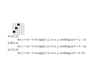
Accumulator Array • at A(1,2) • for y = ax + b we apply 1,2, to x, y, resulting in b = 2 – 1a • at B(2,4) • for y = ax + b we apply 2,4, to x, y, resulting in b = 4 – 2a • at C(3,6) • for y = ax + b we apply 3,6, to x, y, resulting in b = 6 -3a When a = 1 the corresponding value of b = 1 When a = 2 the corresponding value of b = 0 When a = 3 the corresponding value of b = -1 When a = 4 the corresponding value of b = -2 When a = 5 the corresponding value of b = -3 • b = 2 – 1a
Accumulator Array b = 4 – 2a When a = 1 the corresponding value of b = 2 When a = 2 the corresponding value of b = 0 When a = 3 the corresponding value of b = -2 When a = 4 the corresponding value of b = -4 When a = 5 the corresponding value of b = -6 • Since 2 is the highest value of all the numbers in the Accumulator Array, this indicates that A(1,2), and B(2,4) are valid points. • We can now draw a line connecting A and B. The resulting line is y = 2x + 0. • However, this method has its drawbacks. If the line is horizontal, then “a” is 0, and if the line is vertical, then “a” is infinite.
(ak, bk) (a, b) Hough transform • Paul Hough [1962], patented by IBM • How to determine a line ? Tow point A(xi, yi) and B(xj, yj) determine a line • yi = axi + b • yj = axj + b • Line with parameters (a, b) A line is determined by slope-intercept (a, b) yi = Axi + B
(x, y) Problem with y=ax+b • Solution for line function with slope a = • Polar coordinates representation of a line translating Cartesian coordinates (x, y) to Polar coordinates (ρ,θ) Inner product = 0
Hough transform 3 points, A, B and C in polar coordinates, these 3 points will have three curves that intersect at (ρ0,θ0).
Implementing Hough transform 1. Input as Cartesian coordinate entries, “ImgArr[i][j]” 2. Calculate the given point in polar space, we get the curve calculate the values of = xcosθ+ysinθfor all discrete θ 3. Process the results enter into an accumulator array whose size are the number of angles θ and values 4. Updating the accumulator array 5. Detect a peak position to the accumulative array to find potential locations of straight lines
Implementing Hough transform 1. decide on a discrete set of values of θ and to use • 0 and -90θ180 • angles=[-90:180]*pi/180; % 弳度 2. For each edge point, calculate the values of = xcosθ+ysinθfor all discrete θ • [x,y]=find(im); % im is binary, find nonzero • r=floor(x*cos(angles)+y*sin(angles)); % floor: take integers % what’s the dimension of r ?
Implementing Hough transform (cont.) 3. Create an accumulator array whose size are the number of angles θ and values • rmax=max(r( find(r>0) )); • acc=zeros(rmax+1, length(angles)); 4. Updating the accumulator array as we go • for i=1:size(r,1) • for j=1:size(r,2) • if r(i,j)>=0 • acc( r(i,j)+1, j) =acc ( r(i,j)+1, j) +1; • end; end; end; for extra 0
Implementing Hough transform (cont.) • Exercise#1: • c=imread(‘cameraman.tif’); • edge=edge(c, ‘canny’); • According to the previous slides, write a Hough transform MATLAB function • M=max(acc(:)); • [r, theta]=find(acc==M)
Plot the detected line • r=152, theta=169=> index in [-90:180] => θ=169-1-90=78 y Θ=78o Exercise#2: Calculate the coordinate of the green points x
MATLAB line function • line([x1, x2], [y1, y2]) • Which plots in usual Cartesian coordinate (x1, y1) x Exercise#3: Plot your calculated line on the image (x2, y2) y

