Exploring Robust Fitting in Image Processing
350 likes | 376 Vues
Learn about robust fitting techniques in image processing, from affine transformations to RANSAC algorithm for object detection. Discover how to detect objects in images and match features effectively.

Exploring Robust Fitting in Image Processing
E N D
Presentation Transcript
Robust fitting Prof. Noah Snavely CS1114 http://www.cs.cornell.edu/courses/cs1114
Administrivia • A4 due on Friday (please sign up for demo slots) • A5 will be out soon • Prelim 2 is coming up, Tuesday, 4/10
Roadmap • What’s left (next 6.5 weeks): • 2 assignments (A5, A6) • 1 final project • 3 quizzes • 2 prelims
Tricks with convex hull • What else can we do with convex hull? • Answer: sort! • Given a list of numbers (x1, x2, … xn), create a list of 2D points: (x1, x12),(x2, x22), … (xn, xn2) • Find the convex hull of these points – the points will be in sorted order • What does this tell us about the running time of convex hull?
Tricks with convex hull • This is called a reduction from sorting to convex hull
Next couple weeks • How do we detect an object in an image? • Combines ideas from image transformations, least squares, and robustness
Invariant local features • Find features that are invariant to transformations • geometric invariance: translation, rotation, scale • photometric invariance: brightness, exposure, … (Slides courtesy Steve Seitz) Feature Descriptors
Object matching in three steps • Detect features in the template and search images • Match features: find “similar-looking” features in the two images • Find a transformation T that explains the movement of the matched features sift
2D Linear Transformations • Can be represented with a 2D matrix • And applied to a point using matrix multiplication
Image transformations • Rotation is around the point (0, 0) – the upper-left corner of the image • This isn’t really what we want…
Translation • We really want to rotate around the center of the image • Approach: move the center of the image to the origin, rotate, then the center back • (Moving an image is called “translation”) • But translation isn’t linear…
Homogeneous coordinates • Add a 1 to the end of our 2D points (x, y) (x, y, 1) • “Homogeneous” 2D points • We can represent transformations on 2D homogeneous coordinates as 3D matrices
Translation • Other transformations just add an extra row and column with [ 0 0 1 ] scale rotation
Correct rotation • Translate center to origin • Rotate • Translate back to center
Affine transformations • A 2D affine transformation has the form: • Can be thought of as a 2x2 linear transformation plus translation • This will come up again soon in object detection…
Fitting affine transformations • We will fit an affine transformation to a set of feature matches • Problem: there are many incorrect matches
Back to fitting • Simple case: fitting a line
Linear regression • But what happens here? How do we fix this?
Least squares fitting This objective function measures the “goodness” of a hypothesized line
Beyond least squares • We need to change our objective function • Needs to be robust to outliers
Beyond least squares • Idea: count the number of points that are “close” to the line
Testing goodness • Idea: count the number of points that are “close” to the line
Testing goodness • Idea: count the number of points that are “close” to the line Score = 2
Testing goodness • Idea: count the number of points that are “close” to the line
Testing goodness • Idea: count the number of points that are “close” to the line Score = 3
Testing goodness • Idea: count the number of points that are “close” to the line
Testing goodness • Idea: count the number of points that are “close” to the line Score = 7
Testing goodness • How can we tell if a point agrees with a line? • Compute the distance the point and the line, and threshold
Testing goodness • If the distance is small, we call this point an inlier to the line • If the distance is large, it’s an outlier to the line • For an inlier point and a good line, this distance will be close to (but not exactly) zero • For an outlier point or bad line, this distance will probably be large • Objective function: find the line with the most inliers (or the fewest outliers)
Optimizing for inlier count • How do we find the best possible line? Score = 7
Algorithm (RANSAC) • Select two points at random • Solve for the line between those point • Count the number of inliers to the line L • If L has the highest number of inliers so far, save it • Repeat for N rounds, return the best L
Testing goodness • This algorithm is called RANSAC (RANdom SAmple Consensus) – example of a randomized algorithm • Used in an amazing number of computer vision algorithms • Requires two parameters: • The agreement threshold (how close does an inlier have to be?) • The number of rounds (how many do we need?)