Download
1 / 48
480 likes | 526 Vues
Learn about classification and regression, issues, decision tree induction, and more in data analysis. Explore applications like credit approval and medical diagnosis, and understand how classification rules are applied.

E N D
Classification and Prediction • What is classification? What is regression? • Issues regarding classification and prediction • Classification by decision tree induction • Scalable decision tree induction
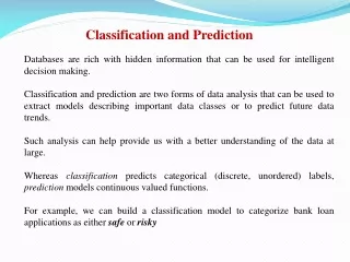
Classification vs. Prediction • Classification: • predicts categorical class labels • classifies data (constructs a model) based on the training set and the values (class labels) in a classifying attribute and uses it in classifying new data • Regression: • models continuous-valued functions, i.e., predicts unknown or missing values • Typical Applications • credit approval • target marketing • medical diagnosis • treatment effectiveness analysis
Why Classification? A motivating application • Credit approval • A bank wants to classify its customers based on whether they are expected to pay back their approved loans • The history of past customers is used to train the classifier • The classifier provides rules, which identify potentially reliable future customers • Classification rule: • If age = “31...40” and income = high then credit_rating = excellent • Future customers • Paul: age = 35, income = high excellent credit rating • John: age = 20, income = medium fair credit rating
Classification—A Two-Step Process • Model construction: describing a set of predetermined classes • Each tuple/sample is assumed to belong to a predefined class, as determined by the class label attribute • The set of tuples used for model construction: training set • The model is represented as classification rules, decision trees, or mathematical formulae • Model usage: for classifying future or unknown objects • Estimate accuracy of the model • The known label of test samples is compared with the classified result from the model • Accuracy rate is the percentage of test set samples that are correctly classified by the model • Test set is independent of training set, otherwise over-fitting will occur
Training Data Classifier (Model) Classification Process (1): Model Construction Classification Algorithms IF rank = ‘professor’ OR years > 6 THEN tenured = ‘yes’
Classifier Testing Data Unseen Data Classification Process (2): Use the Model in Prediction Accuracy=? (Jeff, Professor, 4) Tenured?
Supervised vs. Unsupervised Learning • Supervised learning (classification) • Supervision: The training data (observations, measurements, etc.) are accompanied by labels indicating the class of the observations • New data is classified based on the training set • Unsupervised learning(clustering) • The class labels of training data is unknown • Given a set of measurements, observations, etc. with the aim of establishing the existence of classes or clusters in the data
Issues regarding classification and prediction (1): Data Preparation • Data cleaning • Preprocess data in order to reduce noise and handle missing values • Relevance analysis (feature selection) • Remove the irrelevant or redundant attributes • Data transformation • Generalize and/or normalize data • numerical attribute income categorical {low,medium,high} • normalize all numerical attributes to [0,1)
Issues regarding classification and prediction (2): Evaluating Classification Methods • Predictive accuracy • Speed • time to construct the model • time to use the model • Robustness • handling noise and missing values • Scalability • efficiency in disk-resident databases • Interpretability: • understanding and insight provided by the model • Goodness of rules (quality) • decision tree size • compactness of classification rules
Classification by Decision Tree Induction • Decision tree • A flow-chart-like tree structure • Internal node denotes a test on an attribute • Branch represents an outcome of the test • Leaf nodes represent class labels or class distribution • Decision tree generation consists of two phases • Tree construction • At start, all the training examples are at the root • Partition examples recursively based on selected attributes • Tree pruning • Identify and remove branches that reflect noise or outliers • Use of decision tree: Classifying an unknown sample • Test the attribute values of the sample against the decision tree
Training Dataset This follows an example from Quinlan’s ID3
Output: A Decision Tree for “buys_computer” age? overcast <=30 >40 30..40 student? credit rating? yes no yes fair excellent no yes no yes
Algorithm for Decision Tree Induction • Basic algorithm (a greedy algorithm) • Tree is constructed in a top-down recursive divide-and-conquer manner • At start, all the training examples are at the root • Attributes are categorical (if continuous-valued, they are discretized in advance) • Samples are partitioned recursively based on selected attributes • Test attributes are selected on the basis of a heuristic or statistical measure (e.g., information gain) • Conditions for stopping partitioning • All samples for a given node belong to the same class • There are no remaining attributes for further partitioning – majority voting is employed for classifying the leaf • There are no samples left
Algorithm for Decision Tree Induction (pseudocode) Algorithm GenDecTree(Sample S, Attlist A) • create a node N • If all samples are of the same class C then label N with C; terminate; • If A is empty then label N with the most common class C in S (majority voting); terminate; • Select aA, with the highest information gain; Label N with a; • For each value v of a: • Grow a branch from N with condition a=v; • Let Sv be the subset of samples in S with a=v; • If Sv is empty then attach a leaf labeled with the most common class in S; • Else attach the node generated by GenDecTree(Sv, A-a)
Attribute Selection Measure: Information Gain (ID3/C4.5) • Select the attribute with the highest information gain • Let pi be the probability that an arbitrary tuple in D belongs to class Ci, estimated by |Ci, D|/|D| • Expected information (entropy) needed to classify a tuple in D: • Information needed (after using A to split D into v partitions) to classify D: • Information gained by branching on attribute A
Class P: buys_computer = “yes” Class N: buys_computer = “no” Attribute Selection: Information Gain
Splitting the samples using age age? >40 <=30 30...40 labeled yes
Computing Information-Gain for Continuous-Value Attributes • Let attribute A be a continuous-valued attribute • Must determine the best split point for A • Sort the value A in increasing order • Typically, the midpoint between each pair of adjacent values is considered as a possible split point • (ai+ai+1)/2 is the midpoint between the values of ai and ai+1 • The point with the minimum expected information requirement for A is selected as the split-point for A • Split: • D1 is the set of tuples in D satisfying A ≤ split-point, and D2 is the set of tuples in D satisfying A > split-point
Gain Ratio for Attribute Selection (C4.5) • Information gain measure is biased towards attributes with a large number of values • C4.5 (a successor of ID3) uses gain ratio to overcome the problem (normalization to information gain) • GainRatio(A) = Gain(A)/SplitInfo(A) • Ex. gain_ratio(income) = 0.029/0.926 = 0.031 • The attribute with the maximum gain ratio is selected as the splitting attribute
Gini index (CART, IBM IntelligentMiner) • If a data set D contains examples from n classes, gini index, gini(D) is defined as where pj is the relative frequency of class j in D • If a data set D is split on A into two subsets D1 and D2, the gini index gini(D) is defined as • Reduction in Impurity: • The attribute provides the smallest ginisplit(D) (or the largest reduction in impurity) is chosen to split the node (need to enumerate all the possible splitting points for each attribute)
Gini index (CART, IBM IntelligentMiner) • Ex. D has 9 tuples in buys_computer = “yes” and 5 in “no” • Suppose the attribute income partitions D into 10 in D1: {low, medium} and 4 in D2 but gini{medium,high} is 0.30 and thus the best since it is the lowest • All attributes are assumed continuous-valued • May need other tools, e.g., clustering, to get the possible split values • Can be modified for categorical attributes
Comparing Attribute Selection Measures • The three measures, in general, return good results but • Information gain: • biased towards multivalued attributes • Gain ratio: • tends to prefer unbalanced splits in which one partition is much smaller than the others • Gini index: • biased to multivalued attributes • has difficulty when # of classes is large • tends to favor tests that result in equal-sized partitions and purity in both partitions
Comparison among Splitting Criteria For a 2-class problem:
Overfitting and Tree Pruning • Overfitting: An induced tree may overfit the training data • Too many branches, some may reflect anomalies due to noise or outliers • Poor accuracy for unseen samples • Two approaches to avoid overfitting • Prepruning: Halt tree construction early—do not split a node if this would result in the goodness measure falling below a threshold • Difficult to choose an appropriate threshold • Postpruning: Remove branches from a “fully grown” tree—get a sequence of progressively pruned trees • Use a set of data different from the training data to decide which is the “best pruned tree”
Classification in Large Databases • Classification—a classical problem extensively studied by statisticians and machine learning researchers • Scalability: Classifying data sets with millions of examples and hundreds of attributes with reasonable speed • Why decision tree induction in data mining? • relatively faster learning speed (than other classification methods) • convertible to simple and easy to understand classification rules • can use SQL queries for accessing databases • comparable classification accuracy with other methods
Scalable Decision Tree Induction Methods • SLIQ (EDBT’96 — Mehta et al.) • Builds an index for each attribute and only class list and the current attribute list reside in memory • SPRINT (VLDB’96 — J. Shafer et al.) • Constructs an attribute list data structure • PUBLIC (VLDB’98 — Rastogi & Shim) • Integrates tree splitting and tree pruning: stop growing the tree earlier • RainForest (VLDB’98 — Gehrke, Ramakrishnan & Ganti) • Builds an AVC-list (attribute, value, class label) • BOAT (PODS’99 — Gehrke, Ganti, Ramakrishnan & Loh) • Uses bootstrapping to create several small samples
SLIQ (Supervised Learning In Quest) • Decision-tree classifier for data mining • Design goals: • Able to handle large disk-resident training sets • No restrictions on training-set size
Building tree GrowTree(TrainingData D) Partition(D); Partition(Data D) if(all points in D belong to the same class) then return; for each attribute A do evaluate splits on attribute A; use best split found to partition D into D1 and D2; Partition(D1); Partition(D2);
Data Setup • One list for each attribute • Entries in an Attribute List consist of: • attribute value • class list index • A list for the classes with pointers to the tree nodes • Lists for continuous attributes are in sorted order • Attribute lists may be disk-resident • Class List must be in main memory
Data Setup Class list Attribute lists N1
Evaluating Split Points • Gini Index • if data D contains examples from c classes Gini(D) = 1 - pj2 where pj is the relative frequency of class j in D • If D split into D1 & D2 with n1 & n2 tuples each Ginisplit(D) = n1* gini(D1) + n2* gini(D2) n n • Note: Only class frequencies are needed to compute index
Finding Split Points • For each attribute A do • evaluate splits on attribute A using attribute list • Key idea: To evaluate a split on numerical attributes we need to sort the set at each node. But, if we have all attributes pre-sorted we don’t need to do that at the tree construction phase • Keep split with lowest GINI index
Finding Split Points: Continuous Attrib. • Consider splits of form: value(A) < x • Example: Age < 17 • Evaluate this split-form for every value in an attribute list • To evaluate splits on attribute A for a given tree-node: Initialize class-histograms of left and right children; for each record in the attribute list do find the corresponding entry in Class List and the class and Leaf node evaluate splitting index for value(A) < record.value; update the class histogram in the leaf
N1 GINI Index: und 0 0 1 0.33 3 1 4 3 0.22 1: Age < 20 3: Age < 32 Age < 32 4: Age < 43 0.5 4
Finding Split Points: Categorical Attrib. • Consider splits of the form: value(A) {x1, x2, ..., xn} • Example: CarType {family, sports} • Evaluate this split-form for subsets of domain(A) • To evaluate splits on attribute A for a given tree node: initialize class/value matrix of node to zeroes; for each record in the attribute list do increment appropriate count in matrix; evaluate splitting index for various subsets using the constructed matrix;
class/value matrix Left Child Right Child GINI Index: CarType in {family} GINI = 0.444 CarType in {sports} GINI = 0.333 CarType in {truck} GINI = 0.267
Updating the Class List For each attribute A in a split traverse the attribute list for each value u in the attr list find the corresponding entry in the class list (e) find the new node c to which u belongs update node reference in e to the node corresponding to c • Next step is to update the Class List with the new nodes • Scan the attr list that is used to split and update the corresponding leaf entry in the Class List
Preventing overfitting • A tree T overfits if there is another tree T’ that gives higher error on the training data yet gives lower error on unseen data. • An overfitted tree does not generalize to unseen instances. • Happens when data contains noise or irrelevant attributes and training size is small. • Overfitting can reduce accuracy drastically: • 10-25% as reported in Minger’s 1989 Machine learning
Approaches to prevent overfitting • Two Approaches: • Stop growing the tree beyond a certain point • First over-fit, then post prune. (More widely used) • Tree building divided into phases: • Growth phase • Prune phase • Hard to decide when to stop growing the tree, so second approach more widely used.
Criteria for finding correct final tree size: • Three criteria: • Cross validation with separate test data • Use some criteria function to choose best size • Example: Minimum description length (MDL) criteria • Statistical bounds: use all data for training but apply statistical test to decide right size.
Occam’s Razor • Given two models of similar generalization errors, one should prefer the simpler model over the more complex model • Therefore, one should include model complexity when evaluating a model “entia non sunt multiplicanda praeter ecessitatem,” which translates to: “entities should not be multiplied beyond necessity.”
Minimum Description Length (MDL) • Cost(Model,Data) = Cost(Data|Model) + Cost(Model) • Cost is the number of bits needed for encoding. • Search for the least costly model. • Cost(Data|Model) encodes the misclassification errors. • Cost(Model) uses node encoding (number of children) plus splitting condition encoding.
Encoding data • Assume t records of training data D • First send tree m using L(m) bits • Assume all but the class labels of training data known. • Goal: transmit class labels using L(D|m) • If tree correctly predicts an instance, 0 bits • Otherwise, log k bits where k is number of classes. • Thus, if e errors on training data: total cost • e log k + L(m|M) bits. • Complex tree will have higher L(m) but lower e. • Question: how to encode the tree?
SPRINT • An improvement over SLIQ • Does not need to keep a list in main memory • Attribute lists are extended with class field – no Class list is needed • After a split, the ALs are partitioned. • To split the ALs of the non-split attributes a hash table with the record groups is kept in memory
Pros and Cons of decision trees • Cons • Cannot handle complicated relationship between features • simple decision boundaries • problems with lots of missing data • Pros • Reasonable training time • Fast application • Easy to interpret • Easy to implement • Can handle large number of features
Decision Boundary • Border line between two neighboring regions of different classes is known as decision boundary • Decision boundary is parallel to axes because test condition involves a single attribute at-a-time
x + y < 1 Class = + Class = Oblique Decision Trees • Test condition may involve multiple attributes • More expressive representation • Finding optimal test condition is computationally expensive