Analog Filters: Introduction
Analog Filters: Introduction. Franco Maloberti. Historical Evolution. Frequency and Size. Active filters will achieve ten of GHz in monolitic form. Introduction. An analog filter is the interconnection of components (resistors, capacitors, inductors, active devices)

Analog Filters: Introduction
E N D
Presentation Transcript
Analog Filters: Introduction Franco Maloberti
Historical Evolution Analog Filters: Introduction
Frequency and Size • Active filters will achieve ten of GHz in monolitic form Analog Filters: Introduction
Introduction • An analog filter is the interconnection of components (resistors, capacitors, inductors, active devices) • It has one input (excitation) and one input (response) • It determines a frequency selective transmission. Input Output Analog Filter x(t) y(t) Analog Filters: Introduction
Classification of Systems • Time-Invariant and Time-Varying • The shape of the response does not depends on the time of application of the input • Casual System • The response cannot precede the excitation Analog Filters: Introduction
Classification of Systems • Linear and Non-linear • A system is linear if it satisfies the principle of superposition • Continuous and Discrete-time • In a continuous-time or continuous analog system the variables change continuously with time • In discrete-time or sampled-data systems the variables change at only discrete instants of time Analog Filters: Introduction
Linear Continuous Time-Invariant • If a system is composed by lumped elements (and active devices) • Linear differential equations, constant coefficients • x(t), input, and y(t), output,are current and/or voltages • For a given input and initial conditions the output is completely determined Analog Filters: Introduction
Responses of a linear system • Zero-input response • Is the response obtained when all the inputs are zero. • Depends on the initial charges of capacitors and initial flux of inductors • Zero-state response • Is the response obtained with zero initial conditions • The complete response will be a combination of zero-input and zero-state. Analog Filters: Introduction
Frequency-domain Study • Remember that the Laplace transform of • The equation • Becomes • ICy(s) and ICx(s) accounts for initial conditions Analog Filters: Introduction
Transfer Function • If X(s) is the input and Y(s) the zero-state output • Input voltage, output voltage: voltage TF • Inpur current, output current: Current TF • Input votage output current: Transfer impedance • Input current, ourput voltage: Trasnsfer admittance Analog Filters: Introduction
Transfer Function • Input and output ar normally either voltage or current • Where Y(s) and X(s) are the Laplace transforms of y(t) and x(t) respectively. • In the frequency domain the focus is directed toward • Magnitude and/or Phase on the j axis of s Analog Filters: Introduction
Magnitude and Phase • Magnitude is often expressed in dB • Important is also the group delay • When both magnitude and phase are important the magnitude response is realized first. Then, an additional circuit, the delay equalizer, improves the delay function. Analog Filters: Introduction
Real Transfer Function • The coefficients of the TF are real for a linear, time-invariant lumped network. • Only real or conjugate pairs of complex poles • For stability the zeros of D(s) in the half left plane • D(s) is a Hurwitz polynomial Analog Filters: Introduction
Minimum Phase Filters • When the zeros of N(s) lie on or to the left of the jw-axis H(s) is a minimum phase function. Analog Filters: Introduction
Type of Filters • Low-pass • High-pass • Band-pass • Band-Reject • All-Pass 1 f 0 1 fc f 1 0 fc f 1 0 fc1 fc2 f 0 1 fc fc2 f 0 Analog Filters: Introduction
Approximate Response • Pass-band ripple ap=20Log[Amax/Amin] • Stop-band attenuation, Asb • Transition-band ratio wp, ws Amax Amin Asb wp ws Analog Filters: Introduction
MATLAB • Works with matrices (real, complex or symbolic) • Multiply two polinomials f1(s)=5s3+4s2+2s +1; f2(s)=3s2+5 • clear all; • f1=[5 4 2 1]; • f2 = [3 0 5]; • f3 = conv(f1, f2) 15 12 31 23 10 5 f3(s)=15s5+12s4+ 31s3 + 23s2 + 10s+5 Analog Filters: Introduction
Frequency Scaling • If every inductance and every capacitance of a network is divided by the frequency scaling factor kf, then the network function H(s) becomes H(s/kf). • Xc=1/sC; X’c=1/[s(C/kf)]=1/[C(s/kf)] • XL=sL; X’L=s(L/kf)=L(s/kf) • What occurs at w’ in the original network now will occur at kf w’. Analog Filters: Introduction
Impedance Scaling • All elements with resistance dimension are multiplied by kz • R -> kz R; wL ->kzwL; (Vx=aIcont) a -> a kz • All elements with capacitance dimension are divided by kz • G -> G/kz; wC ->wC /kz; (Ix=bVcont) b -> b/kz • Impedences multiplied by kz • Admittances divided by kz • Dimensionless variables unchanged Analog Filters: Introduction
Normalization and Denormalization • Normalized filters use the key angular frequency of the filter (wp in a low-pass, …) equal to 1. • One of the resistance of the filter is set to 1 • or • One capacitor of the filter is set to 1 • Frequency scaling and impedance scaling are eventually performed at the end of the design process Analog Filters: Introduction
Design of Filters Procedure • Specifications • Kind of network • Input network • Infinite, zero load • Single terminated/Double terminated • Mask of the filter • Magnitude response • Delay response • Other features • Cost, volume, power consumption, temperature drift, aging, … Analog Filters: Introduction
Design of Filters Procedure (ii) • Normalization • Set the value of one key component to 1 • Set the value of one key frequency to 1 • Approximation • To find the transfer function that satisfy the (normalized) amplitude specifications (and, when required, the delay specification. • Many transfer functions achieve the goal. The key task is to select the “cheapest” one Analog Filters: Introduction
Design of Filters Procedure (iii) • Network Synthesis (Realization) • To find a network that realizes the transfer function • Many networks achieve the same transfer function • Active or passive implementation • The behavior of networks implementing the same transfer function can be different (sensitivity, cost, … • Denormalization • Impedance scaling • Frequency scaling • Frequency transformation Analog Filters: Introduction