Download

1 / 52
640 likes | 2.67k Vues
Capacity Planning in Services Industry. Matching Supply and Demand in Service Processes Performance Measures Causes of Waiting Economics of Waiting Management of Waiting Time The Sof-Optics Case. Make to stock vs. Make to Order. Made-to-stock operations (Chapters 6&7)

E N D
Capacity Planning in Services Industry • Matching Supply and Demand in Service Processes • Performance Measures • Causes of Waiting • Economics of Waiting • Management of Waiting Time • The Sof-Optics Case
Make to stock vs. Make to Order • Made-to-stock operations (Chapters 6&7) • Product is manufactured and stocked in advance of demand • Inventory permits economies of scale and protects against stockouts due to variability of inflows and outflows • Make-to-order process (Chapter 8) • Each order is specific, cannot be stored in advance • Process Manger needs to maintain sufficient capacity • Variability in both arrival and processing time • Role of capacity rather than inventory • Safety inventory vs. Safety Capacity • Example: Service operations
Examples • Banks (tellers, ATMs, drive-ins) • Fast food restaurants (counters, drive-ins) • Retail (checkout counters) • Airline (reservation, check-in, takeoff, landing, baggage claim) • Hospitals (ER, OR, HMO) • Service facilities (repair, job shop, ships/trucks load/unload) • Some production systems- to some extend (Dell computer) • Call centers (telemarketing, help desks, 911 emergency)
The DesiTalk Call Center The Call Center Process Sales Reps Processing Calls (Service Process) Incoming Calls (Customer Arrivals) Answered Calls (Customer Departures) Calls on Hold (Service Inventory) Blocked Calls (Due to busy signal) Abandoned Calls (Due to long waits) Calls In Process (Due to long waits)
Service Process Attributes • Ri:customer arrival (inflow) rate inter-arrival time = 1/Ri: • Tp : processing time processing rate per recourse = R’p = 1/Tp • Rp: process capacity with c recourses, Rp=c/Tp • Throughput (flow rate), R = Min(Ri, Rp) Utilization: r= R/Rp Safety Capacity: Rs = Rp-Ri Ti: waiting time in the inflow buffer Ii: number of customers waiting in the inflow buffer K: buffer capacity
Operational Performance Measures • Flow time T = Ti+ Tp • Inventory I = Ii + Ip • Flow Rate R= Min (Ri, Rp) • Stable Process = Ri< Rp,, so that R= Ri • Safety Capacity Rs = Rp - Ri • I = Ri T Ii = Ri Ti Ip = Ri Tp • = Ip/ c = Ri Tp / c = Ri / Rp < 1 • Number of Busy Servers = Ip= c = Ri Tp • Fraction Lost Pb= P(Blocking) = P(Queue = K)
Financial Performance Measures • Sales • Throughput Rate • Abandonment Rate • Blocking Rate • Cost • Capacity utilization • Number in queue / in system • Customer service • Waiting Time in queue /in system
Flow Times with Arrival Every 4 Secs What is the queue size? What is the capacity utilization?
Flow Times with Arrival Every 6 Secs What is the queue size? What is the capacity utilization?
Effect of Variability What is the queue size? What is the capacity utilization?
Effect of Synchronization What is the queue size? What is the capacity utilization?
Conclusion • If inter-arrival and processing times are constant, queues will build up if and only if the arrival rate is greater than the processing rate • If there is (unsynchronized) variability in inter-arrival and/or processing times, queues will build up even if the average arrival rate is less than the average processing rate • If variability in interarrival and processing times can be synchronized (correlated), queues and waiting times will be reduced
Causes of Delays and Queues • High, unsynchronized variability in • - Interarrival times • - Processing times • High capacity utilization ρ= Ri / Rpor low safety capacity • Rs=Ri- Rpdue to : • - High inflow rate Ri • - Low processing rate Rp=c / Tp, which may be due to small-scale c and/or slow speed 1 / Tp
Drivers of Process Performance • Two key drivers of process performance, • Stochastic variability • Capacity utilization • They are determined by two factors: • The mean and variability of interarrival times (measured by total # of arrival over a fixed period of time) 2. The mean and variability of processing times • (measured for different customers) • Variability in the interarrival and processing times can be measured using standard deviation. • Higher standard deviation means greater variability. • Not always an accurate picture of variability • Coefficient of Variation: the ratio of the standard deviation to the mean. Ci = coefficient of variation for interarrival times Cp = coefficient of variation for processing times
The Queue Length Formula Utilization effect Variability effect x Ri / Rp, where Rp = c / Tp Ciand Cp are the Coefficients of Variation (Standard Deviation/Mean) of the inter-arrival and processing times (assumed independent)
Factors affecting Queue Length • This part factor captures the capacity utilization effect, which shows that queue length increases rapidly as the capacity utilization p increases to 1. • The second factor captures the variability effect, which shows that the queue length increases as the variability in interarrival and processing times increases. • Whenever there is variability in arrival or in processing queues will build up and customers will have to wait, even if the processing capacity is not fully utilized.
Average Flow Time T Variability Increases Tp 100% r Utilization (ρ) Throughput- Delay Curve
Example 8.4 • A sample of 10 observations on Interarrival times and processing times • 10,10,2,10,1,3,7,9, 2 • =AVERAGE () Avg. interarrival time = 6 • Ri= 1/6 arrivals / sec. • =STDEV() Std. Deviation = 3.94 • Ci= 3.94/6 = 0.66 • 7,1,7 2,8,7,4,8,5, 1 • Tp= 5 seconds • Rp = 1/5 processes/sec. • Std. Deviation = 2.83 • Cp = 2.83/5 = 0.57 • Ri =1/6 < RP =1/5 R = Ri • = R/ RP = (1/6)/(1/5) = 0.83 • With c = 1, the average number of passengers in queue is as follows: • Ii = [(0.832)/(1-0.83)] ×[(0.662+0.572)/2] = 1.56 • On average 1.56 passengers waiting in line, even though safety capacity is Rs= RP - Ri= 1/5 - 1/6 = 1/30 passenger per second, or 2 per minutes
Example 8.4 • Other performance measures: • Ti=Ii/R = (1.56)(6) = 9.4 seconds • Since TP= 5 T = Ti + TP = 14.4 seconds • Total number of passengers in the process is: I = R T = (1/6) (14.4) = 2.4 • C=2 Rp = 2/5 ρ = (1/6)/(2/5) = 0.42 Ii = 0.08
Exponential Model • In the exponential model, the interarrival and processing times are assumed to be independently and exponentially distributed with means 1/Ri and Tp. • Independence of interarrival and processing times means that the two types of variability are completely unsynchronized. • Complete randomness in interarrival and processing times. • Exponentially distribution is Memoryless: regardless of how long it takes for a person to be processed we would expect that person to spend the mean time in the process before being released.
The Exponential Model • Poisson Arrivals • Infinite pool of potential arrivals, who arrive completely randomly, and independently of one another, at an average rate Ri constant over time • Exponential Processing Time • Completely random, unpredictable, i.e., during processing, the time remaining does not depend on the time elapsed, and has mean Tp • Computations • Ci =Cp= 1 • K = ∞ , use Ii Formula • K < ∞ , use Performance.xls
Example • Interarrival time = 6 secs Ri = 10/min • Tp = 5 secs Rp = 12/min for 1 server and 24 /min for 2 servers • Rs = 12-10 = 2
t≤ t in Exponential Distribution • Mean inter-arrival time = 1/Ri • Probability that the time between two arrivals t is less than or equal to a specific vaule of t • P(t≤ t) = 1 -e-Rit,where e = 2.718282, the base of the natural logarithm • Example 8.5: • If the processing time is exponentially distributed with a mean of 5 seconds, the probability that it will take no more than 3 seconds is 1- e-3/5 = 0.451188 • If the time between consecutive passenger arrival is exponentially distributed with a mean of 6 seconds ( Ri =1/6 passenger per second) • The probability that the time between two consecutive arrivals will exceed 10 seconds is e-10/6 = 0.1888
Performance Improvement Levers • Decrease variability in customer inter-arrival and processing times. • Decrease capacity utilization. • Synchronize available capacity with demand.
Variability Reduction Levers • Customers arrival are hard to control • Scheduling, reservations, appointments, etc…. • Variability in processing time • Increased training and standardization processes • Lower employee turnover rate = more experienced work force • Limit product variety
Capacity Utilization Levers • If the capacity utilization can be decreased, there will also be a decrease in delays and queues. • Since ρ=Ri/RP, to decrease capacity utilization there are two options: • Manage Arrivals: Decrease inflow rate Ri • Manage Capacity: Increase processing rate RP • Managing Arrivals • Better scheduling, price differentials, alternative services • Managing Capacity • Increase scale of the process (the number of servers) • Increase speed of the process (lower processing time)
Synchronizing Capacity with Demand • Capacity Adjustment Strategies • Personnel shifts, cross training, flexible resources • Workforce planning & season variability • Synchronizing of inputs and outputs
Effect of Pooling Ri/2 Server 1 Queue 1 Ri Ri/2 Server 2 Queue 2 Server 1 Ri Queue Server 2
Effect of Pooling • Under Design A, • We have Ri = 10/2 = 5 per minute, and TP= 5 seconds, c =1 and K =50, we arrive at a total flow time of 8.58 seconds • Under Design B, • We have Ri =10 per minute, TP= 5 seconds, c=2 and K=50, we arrive at a total flow time of 6.02 seconds • So why is Design B better than A? • Design A the waiting time of customer is dependent on the processing time of those ahead in the queue • Design B, the waiting time of customer is only partially dependent on each preceding customer’s processing time • Combining queues reduces variability and leads to reduce waiting times
Effect of Buffer Capacity • Process Data • Ri = 20/hour, Tp = 2.5 mins, c = 1, K = # Lines – c • Performance Measures
Economics of Capacity Decisions • Cost of Lost Business Cb • $ / customer • Increases with competition • Cost of Buffer Capacity Ck • $/unit/unit time • Cost of Waiting Cw • $ /customer/unit time • Increases with competition • Cost of Processing Cs • $ /server/unit time • Increases with 1/ Tp • Tradeoff: Choose c, Tp, K • Minimize Total Cost/unit time = Cb Ri Pb + Ck K + Cw I (or Ii) + c Cs
Optimal Buffer Capacity • Cost Data • Cost of telephone line = $5/hour, Cost of server = $20/hour, Margin lost = $100/call, Waiting cost = $2/customer/minute • Effect of Buffer Capacity on Total Cost
Performance Variability • Effect of Variability • Average versus Actual Flow time • Time Guarantee • Promise • Service Level • P(Actual Time Time Guarantee) • Safety Time • Time Guarantee – Average Time • Probability Distribution of Actual Flow Time • P(Actual Time t) = 1 – EXP(- t / T)
Effect of Blocking and Abandonment Blocking: the buffer is full = new arrivals are turned away Abandonment: the customers may leave the process before being served Proportion blocked Pb Proportion abandoning Pa
Net Rate: Ri(1- Pb)(1- Pa)Throughput Rate:R=min[Ri(1- Pb)(1- Pa),Rp] Effect of Blocking and Abandonment
Example 8.8 - DesiCom Call Center • Arrival Rate Ri= 20 per hour=0.33 per min • Processing time Tp =2.5 minutes (24/hr) • Number of servers c=1 • Buffer capacity K=5 • Probability of blocking Pb=0.0771 • Average number of calls on hold Ii=1.52 • Average waiting time in queue Ti=4.94 min • Average total time in the system T=7.44 min • Average total number of customers in the system I=2.29
Example 8.8 - DesiCom Call Center • Throughput Rate • R=min[Ri(1- Pb),Rp]= min[20*(1-0.0771),24] • R=18.46 calls/hour • Server utilization: • R/ Rp=18.46/24=0.769
Capacity Investment Decisions • The Economics of Buffer Capacity • Cost of servers wages =$20/hour • Cost of leasing a telephone line=$5 per line per hour • Cost of lost contribution margin =$100 per blocked call • Cost of waiting by callers on hold =$2 per minute per customer • Total Operating Cost is $386.6/hour
Example 8.10 - The Economics of Processing Capacity • The number of line is fixed: n=6 • The buffer capacity K=6-c
Variability in Process Performance • Why considering the average queue length and waiting time as performance measures may not be sufficient? • Average waiting time includes both customers with very long wait and customers with short or no wait. • We would like to look at the entire probability distribution of the waiting time across all customers. • Thus we need to focus on the upper tail of the probability distribution of the waiting time, not just its average value.
Example 8.11 - WalCo Drugs • One pharmacist, Dave • Average of 20 customers per hour • Dave takes Average of 2.5 min to fill prescription • Process rate 24 per hour • Assume exponentially distributed interarrival and processing time; we have single phase, single server exponential model • Average total process is; • T = 1/(Rp – Ri)= 1/(24 -20) = 0.25 or 15 min
Example 8.11 - Probability distribution of the actual time customer spends in process (obtained by simulation)
Example 8.11 - Probability Distribution Analysis • 65% of customers will spend 15 min or less in process • 95% of customers are served within 40 min • 5% of customers are the ones who will bitterly complain. Imagine if they new that the average customer spends 15 min in the system. • 35% may experience delays longer than Average T,15min
Service Promise:Tduedate ,Service Level & Safety Time • SL; The probability of fulfilling the stated promise. The Firm will set the SL and calculate the Tduedate from the probability distribution of the total time in process (T). • Safety time is the time margin that we should allow over and above the expected time to deliver service in order to ensure that we will be able to meet the required date with high probability • Tduedate = T+Tsafety • Prob(Total time in process<=Tduedate) = SL • Larger SL results in grater probability of fulfilling the promise.
Due Date Quotation • Due Date Quotation is the practice of promising a time frame within which the product will be delivered. • We know that in single-phase single server service process; the Actual total time a customer spends in the process is exponentially distributed with mean T. • SL = Prob(Total time in process<=Tduedate) = 1 – EXP( - Tduedate /T) • Which is the fraction of customers who will no longer be delayed more than promised. • Tduedate = -T ln(1 – SL)
Example 8.12 - WalCo Drug • WalCo has set SL = 0.95 • Assuming total time for customers is exponential • Tduedate = -T ln(1 – SL) • Tduedate = -T ln(0.05) = 3T • Flow time for 95 percentile of exponential distribution is three times the average T • Tduedate = 3 * 15 = 45 • 95% of customers will get served within 45 min • Tduedate = T+Tsafety • Tsafety = 45 – 15 = 30 min • 30 min is the extra margin that WalCo should allow as protection against variability
Relating Utilization and Safety Time: Safety Time Vs. Capacity Utilization • Capacity utilization ρ 60 % 70% 80% 90% • Waiting time Ti 1.5Tp 2.33Tp 4Tp 9Tp • Total flow time T= Ti + Tp 2.5Tp 3.33Tp 5Tp 10Tp • Promised time Tduedate 7.7Tp 10Tp 15Tp 30Tp • Safety time Tsafety = Tduedate – T 5Tp 6.67Tp 10Tp 20Tp • Higher the utilization; Longer the promised time and Safety time • Safety Capacity decreases when capacity utilization increases • Larger safety capacity, the smaller safety time and therefore we can promise a shorter wait