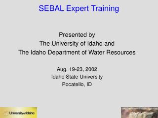
SEBAL Expert Training
SEBAL Expert Training. Presented by The University of Idaho and The Idaho Department of Water Resources Aug. 19-23, 2002 Idaho State University Pocatello, ID. The Trainers. Richard G. Allen, University of Idaho, Kimberly Research Station rallen@kimberly.uidaho.edu Wim M. Bastiaanssen

SEBAL Expert Training
E N D
Presentation Transcript
SEBAL Expert Training Presented by The University of Idaho and The Idaho Department of Water Resources Aug. 19-23, 2002 Idaho State University Pocatello, ID
The Trainers Richard G. Allen,University of Idaho, Kimberly Research Station rallen@kimberly.uidaho.edu Wim M. Bastiaanssen WaterWatch,Wageningen, The Netherlandsw.bastiaanssen@waterwatch.nl Ralf Waters
SEBAL • Surface Energy Balance Algorithm for Land • Developed by • Dr. Wim Bastiaanssen, International Institute for Aerospace Survey and Earth Sciences, The Netherlands • applied in a wide range of international settings • brought to the U.S. by Univ. Idaho in 2000 in cooperation with Idaho Department of Water Resources and NASA/Raytheon
Why Satellites? • Typical method for ET: • weather data are gathered from fixed points -- assumed to extrapolate over large areas • “crop coefficients” assume “well-watered” situation (impacts of stress are difficult to quantify) • Satellite imagery: • energy balance is applied at each “pixel” to map spatial variation • areas where water shortage reduces ET are identified • little or no ground data are required • valid for natural vegetation
Definition of Remote Sensing: The art and science of acquiring information using anon-contact device
SEBAL • UI/IDWR Modifications • digital elevation models for radiation balances in mountains(using slope / aspect / sun angle) • ET at known points tied to alfalfa reference using weather data from Agrimet • testing with lysimeter (ET) data • from Bear River basin (during 2000) • from USDA-ARS at Kimberly (during 2001)
How SEBAL Works SEBAL keys off: • reflectance of light energy • vegetation indices • surface temperature • relative variation in surface temperature • general wind speed (from ground station)
Satellite Compatibility • SEBAL needs both short wave and thermal bands • SEBAL can use images from: • NASA-Landsat (30 m, each 8 or 16 days) - since 1982 • NOAA-AVHRR(advanced very high resolution radiometer) (1 km, daily) - since 1980’s • NASA-MODIS(moderate resolution imaging spectroradiometer) (500 m, daily) - since 1999 • NASA-ASTER(Advanced Spaceborne Thermal Emission and Reflection Radiometer) (15 m, 8 days) - since 1999
Image Processing ERDAS Imagine used to process Landsat images • SEBAL equations programmed and edited in Model Maker function • 20 functions / steps run per image
What Landsat Sees Land Surface Wavelength in Microns Landsat Band 6 is the long-wave “thermal” band and is used for surface temperature
What We Can See With SEBAL Evapotranspiration at time of overpass Oakley Fan, Idaho, July 7, 1989
Uses of ET Maps • Extension / Verification of Pumping or Diversion Records • Recharge to the Snake Plain Aquifer • Feedback to Producers regarding crop health and impacts of irrigation uniformity and adequacy
Why Use SEBAL? • ET via Satellite using SEBAL can provide dependable (i.e. accurate) information • ET can be determined remotely • ET can be determined over large spatial scales • ET can be aggregated over space and time
Future Applications • ET from natural systems • wetlands • rangeland • forests/mountains • use scintillometers and eddy correlation to improve elevation-impacted algorithms in SEBAL • hazardous waste sites • ET from cities • changes in ET as land use changes
R H n ET ET = R - G - H n G Energy Balance for ET ET is calculated as a “residual” of the energy balance Basic Truth: Evaporation consumes Energy The energy balance includes all major sources (Rn) and consumers (ET, G, H) of energy
Surface Radiation Balance Shortwave Radiation Longwave Radiation (1-eo)RL RL aRS (Incident longwave) (reflected longwave) RS RL (Reflected shortwave) (emitted longwave) (Incident shortwave) VegetationSurface Net Surface Radiation = Gains – Losses Rn = (1-a)RS + RL - RL - (1-eo)RL
Preparing the Image • A layered spectral band image is created from the geo-rectified disk using ERDAS Imagine software. • A subset image is created if a smaller area is to be studied.
Band 6 (low & high) Bands 1-5,7 Layering – Landsat 7
Bands 1-7 in order Layering – Landsat 5
Obtaining Header File Information Get the following from the header file: • Overpass date and time • Latitude and Longitude of image center • Sun elevation angle (b) at overpass time • Gain and bias ofr each and (Landsat 7 only)
Method A Applicable for these satellites and formats: • Landsat 5 if original image in NLAPS format • Landsat 7 ETM+ if original image is NLAPS or FAST
GWT Acquiring Header File Information (Landsat 5 - Method A)
Biases Gains Header File for Landsat 7 (bands 1-5,7)
Biases Gains Low gain High gain Header File for Landsat 7 (band 6)
DOY GWT Acquiring Header File Information (Method B)
Calculating the Wind Speed for the Time of the Image For August 22, 2000: image time is 17:57 GMT Apply the correction: timage (Local Time) = 17:57 – 7:00 = 10:57 am Δt = 1 t1 = int 10+57/60 + ½ - 0 (1) + 1 = 12 hours 1
Estimate Wind Speed at 10:57 am Interpolate between the value for 12:00 (1.4 m/s) and the value for 13:00 (1.9 m/s) • U = 1.4+(1.9-1.4)[(10+57/60) – (10+1/2)] = 1.63 m/s • To estimate ETr for 10:57 AM: Interpolate between the values for 12:00 (.59) and for 13:00 (.72) • ETr = .59+(.72-.59) [(10+57/60) – (10+1/2)] = 0.65 mm/hr
Surface Radiation Balance Shortwave Radiation Longwave Radiation RS RL (1-eo)RL RL (Incident shortwave) (Incident longwave) (reflected longwave) (emitted longwave) aRS (Reflected shortwave) VegetationSurface Net Surface Radiation = Gains – Losses Rn = (1-a)RS + RL - RL - (1-eo)RL
a model_04 RS↓ calculator RL↑ model_09 RL↓ calculator atoa model_03 TS model_08 eo model_06 rl model_02 NDVI SAVI LAI model_05 Tbb model_07 Ll model_01 Flow Chart – Net Surface Radiation Rn = (1-a)RS↓ + RL↓ - RL↑ - (1-e0)RL↓
Radiance Equation for Landsat 7 Ll = (Gain × DN) + Bias
Enter values from Table 6.1 in Appendix 6 Model 01 – Radiance for Landsat 5