SL and LL visualizations

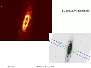
1. SL and LL visualizations 1 15 Jan 2004 SINGS Tucson Meeting - DAD

2. 2 15 Jan 2004 SINGS Tucson Meeting - DAD

3. SL S/N 3 15 Jan 2004 SINGS Tucson Meeting - DAD

4. SL S/N 4 15 Jan 2004 SINGS Tucson Meeting - DAD

5. SH lines 5 15 Jan 2004 SINGS Tucson Meeting - DAD

6. LH lines 6 15 Jan 2004 SINGS Tucson Meeting - DAD

7. LH lines 7 15 Jan 2004 SINGS Tucson Meeting - DAD

8. LL cut 8 15 Jan 2004 SINGS Tucson Meeting - DAD

9. IRS sensitivity 9 15 Jan 2004 SINGS Tucson Meeting - DAD

10. 10 15 Jan 2004 SINGS Tucson Meeting - DAD

11. I've taken the ISO 7 and 15 micron maps for N6946, and used my SED models, to predict the surface brightness at IRS LL wavelengths. The first plot displays the (S/N) spectra from the 11x79 different 4.8" pixels that lie within the 1'x6.4' IRS SED strip (see example image at 27.0 microns). The largest-valued spectra come from the nucleus, whereas the weakest spectra represent the fainter disk. I am assuming the pre-flight sensitivity is applicable (1sigma sensitivity). LL Simulations 11 15 Jan 2004 SINGS Tucson Meeting - DAD

12. The second plot displays the (S/N) spectra you would get if binning was carried out 2x2 spatially, and collapsing spectrally by combining five spectral elements into one (see example image at 28.0 microns). The lines represent spectra from 5x39 different 9.6" pixels that lie with the strip. LL Simulations 12 15 Jan 2004 SINGS Tucson Meeting - DAD

13. MIPS SED Simulations I've taken the ISO 7 and 15 micron maps for N6946, and used my SED models, to predict the surface brightness at MIPS SED wavelengths. The first plot displays the (S/N) spectra from the 6x43 different 9.9" pixels that lie within the 1'x7' MIPS SED strip (see example image at 75.4 microns). The largest-valued spectra come from the nucleus, whereas the weakest spectra represent the fainter disk. 13 15 Jan 2004 SINGS Tucson Meeting - DAD

14. LL Simulations The second plot displays the (S/N) spectra you would get if binning was carried out 2x2 spatially, and collapsing spectrally by combining five 1.7 micron pixels into 8.5 micron pixels (see example image at 75.4 microns). The lines represent spectra from 3x22 different 19.8" pixels that lie with the strip. I am assuming the conservative end of Chad's recent sensitivity range is applicable: 3sigma=36-45 mJy (3sigma=3.2 MJy/sr). 14 15 Jan 2004 SINGS Tucson Meeting - DAD

15. The second plot displays the (S/N) spectra you would get if binning was carried out 2x2 spatially, and collapsing spectrally by combining five spectral elements into one (see example image at 28.0 microns). The lines represent spectra from 5x39 different 9.6" pixels that lie with the strip. LL Simulations 15 15 Jan 2004 SINGS Tucson Meeting - DAD

16. The second plot displays the (S/N) spectra you would get if binning was carried out 2x2 spatially, and collapsing spectrally by combining five spectral elements into one (see example image at 28.0 microns). The lines represent spectra from 5x39 different 9.6" pixels that lie with the strip. LL Simulations 16 15 Jan 2004 SINGS Tucson Meeting - DAD

17. The second plot displays the (S/N) spectra you would get if binning was carried out 2x2 spatially, and collapsing spectrally by combining five spectral elements into one (see example image at 28.0 microns). The lines represent spectra from 5x39 different 9.6" pixels that lie with the strip. MIPS SED Simulations 17 15 Jan 2004 SINGS Tucson Meeting - DAD