Datalog
Datalog. Logical Rules Recursion SQL-99 Recursion. Logic As a Query Language. If-then logical rules have been used in many systems. Most important today: EII (Enterprise Information Integration). Nonrecursive rules are equivalent to the core relational algebra.

Datalog
E N D
Presentation Transcript
Datalog Logical Rules Recursion SQL-99 Recursion
Logic As a Query Language • If-then logical rules have been used in many systems. • Most important today: EII (Enterprise Information Integration). • Nonrecursive rules are equivalent to the core relational algebra. • Recursive rules extend relational algebra --- have been used to add recursion to SQL-99.
A Logical Rule • Our first example of a rule uses the relations: • Frequents(customer,rest), • Likes(customer,soda), and • Sells(rest,soda,price). • The rule is a query asking for “happy” customers --- those that frequent a rest that serves a soda that they like.
Anatomy of a Rule Happy(c) <- Frequents(c,rest) AND Likes(c,soda) AND Sells(rest,soda,p)
Head = “consequent,” a single sub-goal Body = “antecedent” = AND of sub-goals. Read this symbol “if” Anatomy of a Rule Happy(c) <- Frequents(c,rest) AND Likes(c,soda) AND Sells(rest,soda,p)
sub-goals Are Atoms • An atom is a predicate, or relation name with variables or constants as arguments. • The head is an atom; the body is the AND of one or more atoms. • Convention: Predicates begin with a capital, variables begin with lower-case.
Example: Atom Sells(rest, soda, p)
The predicate = name of a relation Arguments are variables Example: Atom Sells(rest, soda, p)
Interpreting Rules • A variable appearing in the head is called distinguished ; • otherwise it is nondistinguished.
Interpreting Rules • Rule meaning: • The head is true of the distinguished variables • if there exist values of the nondistinguished variables • that make all sub-goals of the body true.
Example: Interpretation Happy(c) <- Frequents(c,rest) AND Likes(c,soda) AND Sells(rest,soda,p) Interpretation: customer d is happy if there exist a rest, a soda, and a price p such that c frequents the rest, likes the soda, and the rest sells the soda at price p.
Distinguished variable Nondistinguished variables Example: Interpretation Happy(c) <- Frequents(c,rest) AND Likes(c,soda) AND Sells(rest,soda,p) Interpretation: customer d is happy if there exist a rest, a soda, and a price p such that c frequents the rest, likes the soda, and the rest sells the soda at price p.
Arithmetic sub-goals • In addition to relations as predicates, a predicate for a sub-goal of the body can be an arithmetic comparison. • We write such sub-goals in the usual way, e.g.: x < y.
Example: Arithmetic • A soda is “cheap” if there are at least two rests that sell it for under $1. • Figure out a rule that would determine whether a soda is cheap or not.
Example: Arithmetic Cheap(soda) <- Sells(rest1,soda,p1) AND Sells(rest2,soda,p2) AND p1 < 1.00 AND p2 < 1.00 AND rest1 <> rest2
Negated sub-goals • We may put “NOT” in front of a sub-goal, to negate its meaning.
Negated sub-goals • Example: • Think of Arc(a,b) as arcs in a graph. • S(x,y) says the graph is not transitive from x to y ; i.e., there is a path of length 2 from x to y, but no arc from x to y. S(x,y) <- Arc(x,z) AND Arc(z,y) AND NOT Arc(x,y)
Algorithms for Applying Rules • Two approaches: • Variable-based : Consider all possible assignments to the variables of the body. If the assignment makes the body true, add that tuple for the head to the result. • Tuple-based : Consider all assignments of tuples from the non-negated, relational sub-goals. If the body becomes true, add the head’s tuple to the result.
Example: Variable-Based --- 1 S(x,y) <- Arc(x,z) AND Arc(z,y) AND NOT Arc(x,y) • Arc(1,2) and Arc(2,3) are the only tuples in the Arc relation. • Only assignments to make the first sub-goal Arc(x,z) true are: • x = 1; z = 2 • x = 2; z = 3
Example: Variable-Based; x=1, z=2 S(x,y) <- Arc(x,z) AND Arc(z,y) AND NOT Arc(x,y) 1 1 2 2 1
3 3 3 3 is the only value of y that makes all three sub-goals true. Makes S(1,3) a tuple of the answer Example: Variable-Based; x=1, z=2 S(x,y) <- Arc(x,z) AND Arc(z,y) AND NOT Arc(x,y) 1 1 2 2 1
Example: Variable-Based; x=2, z=3 S(x,y) <- Arc(x,z) AND Arc(z,y) AND NOT Arc(x,y) 2 2 3 3 2
Thus, no contribution to the head tuples; S = {(1,3)} Example: Variable-Based; x=2, z=3 S(x,y) <- Arc(x,z) AND Arc(z,y) AND NOT Arc(x,y) 2 2 3 3 2 No value of y makes Arc(3,y) true.
Tuple-Based Assignment • Start with the non-negated, relational sub-goals only. • Consider all assignments of tuples to these sub-goals. • Choose tuples only from the corresponding relations. • If the assigned tuples give a consistent value to all variables and make the other sub-goals true, add the head tuple to the result.
Example: Tuple-Based S(x,y) <- Arc(x,z) AND Arc(z,y) AND NOT Arc(x,y) Only possible values Arc(1,2), Arc(2,3) • Four possible assignments to first two sub-goals: Arc(x,z) Arc(z,y) (1,2) (1,2) (1,2) (2,3) (2,3) (1,2) (2,3) (2,3)
Only assignment with consistent z-value. Since it also makes NOT Arc(x,y) true, add S(1,3) to result. Example: Tuple-Based S(x,y) <- Arc(x,z) AND Arc(z,y) AND NOT Arc(x,y) Only possible values Arc(1,2), Arc(2,3) • Four possible assignments to first two sub-goals: Arc(x,z) Arc(z,y) (1,2) (1,2) (1,2) (2,3) (2,3) (1,2) (2,3) (2,3) These two rows are invalid since z can’t be(3 and 1) or (3 and 2)simultaneously.
Datalog Programs • A Datalog program is a collection of rules. • In a program, predicates can be either • EDB = Extensional Database • = stored table. • IDB = Intensional Database • = relation defined by rules. • Never both! No EDB in heads.
Evaluating Datalog Programs • As long as there is no recursion, • we can pick an order to evaluate the IDB predicates, • so that all the predicates in the body of its rules have already been evaluated. • If an IDB predicate has more than one rule, • each rule contributes tuples to its relation.
Example: Datalog Program • Using following EDB find all the manufacturers of sodas Joe doesn’t sell: • Sells(rest, soda, price) and • sodas(name, manf). JoeSells(s) <- Sells(’Joe’’s rest’, s, p) Answer(m) <- Sodas(s,m) AND NOT JoeSells(s)
Expressive Power of Datalog • Without recursion, • Datalog can express all and only the queries of core relational algebra. • The same as SQL select-from-where, without aggregation and grouping.
Expressive Power of Datalog • But with recursion, • Datalog can express more than these languages. • Yet still not Turing-complete.
Recursive Example:Generalized Cousins • EDB: Parent(c,p) = p is a parent of c. • Generalized cousins: people with common ancestors one or more generations back. • Note: We are all cousins according to this definition.
Recursive Example Sibling(x,y) <- Parent(x,p) AND Parent(y,p) AND x<>y Cousin(x,y) <- Sibling(x,y) Cousin(x,y) <- Parent(x,xParent) AND Parent(y,yParent) AND Cousin(xParent,yParent)
Definition of Recursion • Form a dependency graph whose nodes = IDB predicates. • Arc X ->Y if and only if • there is a rule with X in the head and Y in the body. • Cycle = recursion; • No cycle = no recursion.
Example: Dependency Graphs Cousin Answer Sibling JoeSells Recursive Non-recursive
Evaluating Recursive Rules • The following works when there is no negation: • Start by assuming all IDB relations are empty. • Repeatedly evaluate the rules using the EDB and the previous IDB, to get a new IDB. • End when no change to IDB.
The “Naïve” Evaluation Algorithm Start: IDB = 0 Apply rules to IDB, EDB no yes Change to IDB? done
Example: Evaluation of Cousin • Remember the rules: Sibling(x,y) <- Parent(x,p) AND Parent(y,p) AND x<>y Cousin(x,y) <- Sibling(x,y) Cousin(x,y) <- Parent(x,xParent) AND Parent(y,yParent) AND Cousin(xParent,yParent)
Semi-naive Evaluation • Since the EDB never changes, • on each round we only get new IDB tuples if we use at least one IDB tuple that was obtained on the previous round. • Saves work; lets us avoid rediscovering most known facts. • A fact could still be derived in a second way.
Example: Evaluation of Cousin • We’ll proceed in rounds to infer • Sibling facts (red) • and Cousin facts (green).
Parent Data: Parent Above Child The parent data, and edge goes downward from a parent to child. Exercises:1. List some of the parent-child relationships. 2. What is contained in the Sibling and Cousin data? a d b c e f g h j k i
Parent Data: Parent Above Child Exercise: 1. What do you expect after first round? a d b c e f g h j k i
Sibling and Cousin are presumed empty. Cousin remains empty since it depends on Sibling and Sibling is empty. Exercise: What do you expect in the next round? Round 1 a d b c e f g h j k i
Sibling facts remain unchanged because Sibling is not recursive. First execution of the Cousin rule “duplicates” the Sibling facts as Cousin facts (shown in green). Exercise: What do you expect in the next round? Round 2 a d b c e f g h j k i
The execution of the non-recursive Cousin rule gives us nothing However, the recursive call gives us several pairs (shown in bolder green). Exercise: What do you expect in the next round? Round 3 a d b c e f g h j k i
The execution of the non-recursive Cousin rule still gives us nothing However, the recursive call gives us several pairs (shown in even bolder green). Exercise: What do you expect in the next round? Round 4 a d b c e f g h j k i
Done! a d b c e f g h j k i Now we are done!
Recursion Plus Negation • “Naïve” and “Semi-Naïve” evaluation doesn’t work when there are negated sub-goals. • Discovering IDB tuples on one route can decrease the IDB tuples on the next route. • Losing IDB tuples on one route can yield more tuples on the next route.
Recursion Plus Negation • In fact, negation wrapped in a recursion makes no sense in general. • Even when recursion and negation are separate, we can have ambiguity about the correct IDB relations.
Problematic Recursive Negation P(x) <- Q(x) AND NOT P(x) EDB: Q(1), Q(2) Initial: P = { } Round 1: P = {(1), (2)} // From Q(1) & Q(2) Round 2: P = { } // From NOT(P(1)) & NOT(P(2)) Round 3: P = {(1), (2)} // From Q(1) & Q(2) Round n: etc., etc. …