Download
1 / 51
510 likes | 657 Vues
Datalog. Logical Rules Recursion. Logic As a Query Language. If-then logical rules have been used in many systems. Important example : EII (Enterprise Information Integration). Nonrecursive rules are equivalent to the core relational algebra.

E N D
Datalog Logical Rules Recursion
Logic As a Query Language • If-then logical rules have been used in many systems. • Important example: EII (Enterprise Information Integration). • Nonrecursive rules are equivalent to the core relational algebra. • Recursive rules extend relational algebra and appear in SQL-99.
Example: Enterprise Integration • Goal: integrated view of the menus at many bars Sells(bar, beer, price). • Joe has data JoeMenu(beer, price). • Approach 1: Describe Sells in terms of JoeMenu and other local data sources. Sells(’Joe’’s Bar’, b, p) <- JoeMenu(b, p)
EII – (2) • Approach 2: Describe how JoeMenu can be used as a view to help answer queries about Sells and other relations. JoeMenu(b, p) <- Sells(’Joe’’s Bar’, b, p) • More about information integration later.
A Logical Rule • Our first example of a rule uses the relations Frequents(drinker, bar), Likes(drinker, beer), and Sells(bar, beer, price). • The rule is a query asking for “happy” drinkers --- those that frequent a bar that serves a beer that they like.
Head = consequent, a single subgoal Body = antecedent = AND of subgoals. Read this symbol “if” Anatomy of a Rule Happy(d) <- Frequents(d,bar) AND Likes(d,beer) AND Sells(bar,beer,p)
Subgoals Are Atoms • An atom is a predicate, or relation name with variables or constants as arguments. • The head is an atom; the body is the AND of one or more atoms. • Convention: Predicates begin with a capital, variables begin with lower-case.
The predicate = name of a relation Arguments are variables (or constants). Example: Atom Sells(bar, beer, p)
Interpreting Rules • A variable appearing in the head is distinguished; otherwise it is nondistinguished. • Rule meaning: The head is true for given values of the distinguished variables if there exist values of the nondistinguished variables that make all subgoals of the body true.
Distinguished variable Nondistinguished variables Example: Interpretation Happy(d) <- Frequents(d,bar) AND Likes(d,beer) AND Sells(bar,beer,p) Interpretation: drinker d is happy if there exist a bar, a beer, and a price p such that d frequents the bar, likes the beer, and the bar sells the beer at price p.
Applying a Rule • Approach 1: consider all combinations of values of the variables. • If all subgoals are true, then evaluate the head. • The resulting head is a tuple in the result.
Example: Rule Evaluation Happy(d) <- Frequents(d,bar) AND Likes(d,beer) AND Sells(bar,beer,p) FOR (each d, bar, beer, p) IF (Frequents(d,bar), Likes(d,beer), and Sells(bar,beer,p) are all true) add Happy(d) to the result • Note: set semantics so add only once.
A Glitch (Fixed Later) • Relations are finite sets. • We want rule evaluations to be finite and lead to finite results. • “Unsafe” rules like P(x)<-Q(y) have infinite results, even if Q is finite. • Even P(x)<-Q(x) requires examining an infinity of x-values.
Applying a Rule – (2) • Approach 2: For each subgoal, consider all tuples that make the subgoal true. • If a selection of tuples define a single value for each variable, then add the head to the result. • Leads to finite search for P(x)<-Q(x), but P(x)<-Q(y) is problematic.
Example: Rule Evaluation – (2) Happy(d) <- Frequents(d,bar) AND Likes(d,beer) AND Sells(bar,beer,p) FOR (each f in Frequents, i in Likes, and s in Sells) IF (f[1]=i[1] and f[2]=s[1] and i[2]=s[2]) add Happy(f[1]) to the result
Arithmetic Subgoals • In addition to relations as predicates, a predicate for a subgoal of the body can be an arithmetic comparison. • We write arithmetic subgoals in the usual way, e.g., x < y.
Example: Arithmetic • A beer is “cheap” if there are at least two bars that sell it for under $2. Cheap(beer) <- Sells(bar1,beer,p1) AND Sells(bar2,beer,p2) AND p1 < 2.00 AND p2 < 2.00 AND bar1 <> bar2
Negated Subgoals • NOT in front of a subgoal negates its meaning. • Example: Think of Arc(a,b) as arcs in a graph. • S(x,y) says the graph is not transitive from x to y ; i.e., there is a path of length 2 from x to y, but no arc from x to y. S(x,y) <- Arc(x,z) AND Arc(z,y) AND NOT Arc(x,y)
Safe Rules • A rule is safe if: • Each distinguished variable, • Each variable in an arithmetic subgoal, and • Each variable in a negated subgoal, also appears in a nonnegated, relational subgoal. • Safe rules prevent infinite results.
Example: Unsafe Rules • Each of the following is unsafe and not allowed: • S(x) <- R(y) • S(x) <- R(y) AND NOT R(x) • S(x) <- R(y) AND x < y • In each case, an infinity of x ’s can satisfy the rule, even if R is a finite relation.
An Advantage of Safe Rules • We can use “approach 2” to evaluation, where we select tuples from only the nonnegated, relational subgoals. • The head, negated relational subgoals, and arithmetic subgoals thus have all their variables defined and can be evaluated.
Datalog Programs • Datalog program = collection of rules. • In a program, predicates can be either • EDB = Extensional Database = stored table. • IDB = Intensional Database = relation defined by rules. • Never both! No EDB in heads.
Evaluating Datalog Programs • As long as there is no recursion, we can pick an order to evaluate the IDB predicates, so that all the predicates in the body of its rules have already been evaluated. • If an IDB predicate has more than one rule, each rule contributes tuples to its relation.
Example: Datalog Program • Using EDB Sells(bar, beer, price) and Beers(name, manf), find the manufacturers of beers Joe doesn’t sell. JoeSells(b) <- Sells(’Joe’’s Bar’, b, p) Answer(m) <- Beers(b,m) AND NOT JoeSells(b)
Example: Evaluation • Step 1: Examine all Sells tuples with first component ’Joe’’s Bar’. • Add the second component to JoeSells. • Step 2: Examine all Beers tuples (b,m). • If b is not in JoeSells, add m to Answer.
Expressive Power of Datalog • Without recursion, Datalog can express all and only the queries of core relational algebra. • The same as SQL select-from-where, without aggregation and grouping. • But with recursion, Datalog can express more than these languages. • Yet still not Turing-complete.
Recursive Example • EDB: Par(c,p) = p is a parent of c. • Generalized cousins: people with common ancestors one or more generations back: Sib(x,y) <- Par(x,p) AND Par(y,p) AND x<>y Cousin(x,y) <- Sib(x,y) Cousin(x,y) <- Par(x,xp) AND Par(y,yp) AND Cousin(xp,yp)
Definition of Recursion • Form a dependency graph whose nodes = IDB predicates. • Arc X ->Y if and only if there is a rule with X in the head and Y in the body. • Cycle = recursion; no cycle = no recursion.
Example: Dependency Graphs Cousin Answer Sib JoeSells Recursive Nonrecursive
Evaluating Recursive Rules • The following works when there is no negation: • Start by assuming all IDB relations are empty. • Repeatedly evaluate the rules using the EDB and the previous IDB, to get a new IDB. • End when no change to IDB.
The “Naïve” Evaluation Algorithm Start: IDB = 0 Apply rules to IDB, EDB no yes Change to IDB? done
Seminaive Evaluation • Since the EDB never changes, on each round we only get new IDB tuples if we use at least one IDB tuple that was obtained on the previous round. • Saves work; lets us avoid rediscovering most known facts. • A fact could still be derived in a second way.
Example: Evaluation of Cousin • We’ll proceed in rounds to infer Sib facts (red) and Cousin facts (green). • Remember the rules: Sib(x,y) <- Par(x,p) AND Par(y,p) AND x<>y Cousin(x,y) <- Sib(x,y) Cousin(x,y) <- Par(x,xp) AND Par(y,yp) AND Cousin(xp,yp)
Round 1 Round 2 Round 3 Round 4 Par Data: Parent Above Child Sib(x,y) <- Par(x,p) AND Par(y,p) AND x<>y Cousin(x,y) <- Par(x,xp) AND Par(y,yp) AND Cousin(xp,yp) Cousin(x,y) <- Sib(x,y) a d b c e f g h j k i
SQL-99 Recursion • Datalog recursion has inspired the addition of recursion to the SQL-99 standard. • Tricky, because SQL allows negation grouping-and-aggregation, which interact with recursion in strange ways.
Form of SQL Recursive Queries WITH <stuff that looks like Datalog rules> <a SQL query about EDB, IDB> “Datalog rule” = [RECURSIVE] <name>(<arguments>) AS <query>
Like Sib(x,y) <- Par(x,p) AND Par(y,p) AND x <> y Example: SQL Recursion – (1) • Find Sally’s cousins, using SQL like the recursive Datalog example. • Par(child,parent) is the EDB. WITH Sib(x,y) AS SELECT p1.child, p2.child FROM Par p1, Par p2 WHERE p1.parent = p2.parent AND p1.child <> p2.child;
Required – Cousin is recursive Reflects Cousin(x,y) <- Sib(x,y) Reflects Cousin(x,y) <- Par(x,xp) AND Par(y,yp) AND Cousin(xp,yp) Example: SQL Recursion – (2) WITH … RECURSIVE Cousin(x,y) AS (SELECT * FROM Sib) UNION (SELECT p1.child, p2.child FROM Par p1, Par p2, Cousin WHERE p1.parent = Cousin.x AND p2.parent = Cousin.y);
Example: SQL Recursion – (3) • With those definitions, we can add the query, which is about the virtual view Cousin(x,y): SELECT y FROM Cousin WHERE x = ’Sally’;
Legal SQL Recursion • It is possible to define SQL recursions that do not have a meaning. • The SQL standard restricts recursion so there is a meaning. • And that meaning can be obtained by seminaïve evaluation.
Example: Meaningless Recursion • EDB: P(x) = {(1)}. • IDB: Q(x) <- P(x) AND NOT Q(x). • Is (1) in Q(x)? • If so, the recursive rule says it is not. • If not, the recursive rule says it is.
Plan to Explain Legal SQL Recursion • Define “monotone” recursions. • Define a “stratum graph” to represent the connections among subqueries. • Define proper SQL recursions in terms of the stratum graph.
Monotonicity • If relation P is a function of relation Q (and perhaps other relations), we say P is monotone in Q if inserting tuples into Q cannot cause any tuple to be deleted from P. • Examples: • P = Q∪R. • P = σa =10(Q ).
Example: Nonmonotonicity SELECT AVG(price) FROM Sells WHERE bar = ’Joe’’s Bar’; is not monotone in Sells. • Inserting a Joe’s-Bar tuple into Sells usually changes the average price and thus deletes the old average price.
Stratum Graph • Nodes = • IDB relations declared in WITH clause. • Subqueries in the body of the “rules.” • Includes subqueries at any level of nesting.
Stratum Graph – (2) • Arcs P ->Q : • P is a rule head and Q is a relation in the FROM list (not of a subquery). • P is a rule head and Q is an immediate subquery of that rule. • P is a subquery, and Q is a relation in its FROM or an immediate subquery (like 1 and 2). • Put “–” on an arc if P is not monotone in Q.
Stratified SQL • A SQL recursion is stratified if there is a finite bound on the number of – signs along any path in its stratum graph. • Including paths with cycles. • Legal SQL recursion = recursion with a stratified stratum graph.
Subquery S1 Subquery S2 Example: Stratum Graph • In our Cousin example, the structure of the rules was: Sib = … Cousin = ( … FROM Sib ) UNION ( … FROM Cousin … )
The Graph No “–” at all, so surely stratified. Sib Cousin S1 S2
Can delete a tuple from Cousin Inserting a tuple into S2 Nonmonotone Example • Change the UNION in the Cousin example to EXCEPT: Sib = … Cousin = ( … FROM Sib ) EXCEPT ( … FROM Cousin … ) Subquery S1 Subquery S2