Linear Regression and Correlation in Data Analysis
Learn about linear regression and correlation, including least squares estimation, residuals, correlation coefficient, and coefficient of determination. Explore practical examples and inference methods. Enhance your data analysis skills now!

Linear Regression and Correlation in Data Analysis
E N D
Presentation Transcript
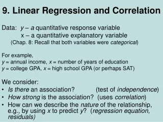
Linear Regression/Correlation • Quantitative Explanatory and Response Variables • Goal: Test whether the level of the response variable is associated with (depends on) the level of the explanatory variable • Goal: Measure the strength of the association between the two variables • Goal: Use the level of the explanatory to predict the level of the response variable
Linear Relationships • Notation: • Y: Response (dependent, outcome) variable • X: Explanatory (independent, predictor) variable • Linear Function (Straight-Line Relation): • Y = a + b X (Plot Y on vertical axis, X horizontal) • Slope (b): The amount Y changes when X increases by 1 • b > 0 Line slopes upward (Positive Relation) • b = 0 Line is flat (No linear Relation) • b < 0 Line slopes downward (Negative Relation) • Y-intercept (a): Y level when X=0
Example: Service Pricing • Internet History Resources (New South Wales Family History Document Service) • Membership fee: $20A • 20¢ ($0.20A) per image viewed • Y = Total cost of service • X = Number of images viewed • a = Cost when no images viewed • b = Incremental Cost per image viewed • Y = a + b X = 20+0.20X
Probabilistic Models • In practice, the relationship between Y and X is not “perfect”. Other sources of variation exist. We decompose Y into 2 components: • Systematic Relationship with X: a + bX • Random Error: e • Random respones can be written as the sum of the systematic (also thought of as the mean) and random components: Y = a + bX + e • The (conditional on X) mean response is: • E(Y) = a + bX
Least Squares Estimation • Problem: a, b are unknown parameters, and must be estimated and tested based on sample data. • Procedure: • Sample n individuals, observing X and Y on each one • Plot the pairs Y (vertical axis) versus X (horizontal) • Choose the line that “best fits” the data. • Criteria: Choose line that minimizes sum of squared vertical distances from observed data points to line. Least Squares Prediction Equation:
Example - Pharmacodynamics of LSD • Response (Y) - Math score (mean among 5 volunteers) • Predictor (X) - LSD tissue concentration (mean of 5 volunteers) • Raw Data and scatterplot of Score vs LSD concentration: Source: Wagner, et al (1968)
Example - Pharmacodynamics of LSD (Column totals given in bottom row of table)
Example - Retail Sales • U.S. SMSA’s • Y = Per Capita Retail Sales • X = Females per 100 Males
Residuals • Residuals (aka Errors): Difference between observed values and predicted values: • Error sum of squares: • Estimate of (conditional) standard deviation of Y:
Linear Regression Model • Data: Y = a + b X + e • Mean: E(Y) = a + b X • Conditional Standard Deviation: s • Error terms (e) are assumed to be independent and normally distributed
Correlation Coefficient • Slope of the regression describes the direction of association (if any) between the explanatory (X) and response (Y). Problems: • The magnitude of the slope depends on the units of the variables • The slope is unbounded, doesn’t measure strength of association • Some situations arise where interest is in association between variables, but no clear definition of X and Y • Population Correlation Coefficient: r • Sample Correlation Coefficient: r
Correlation Coefficient • Pearson Correlation: Measure of strength of linear association: • Does not delineate between explanatory and response variables • Is invariant to linear transformations of Y and X • Is bounded between -1 and 1 (higher values in absolute value imply stronger relation) • Same sign (positive/negative) as slope
Example - Pharmacodynamics of LSD • Using formulas for standard deviation from beginning of course: sX = 1.935 and sY = 18.611 • From previous calculations: b = -9.01 This represents a strong negative association between math scores and LSD tissue concentration
Coefficient of Determination • Measure of the variation in Y that is “explained” by X • Step 1: Ignoring X, measure the total variation in Y (around its mean): • Step 2: Fit regression relating Y to X and measure the unexplained variation in Y (around its predicted values): • Step 3: Take the difference (variation in Y “explained” by X), and divide by total:
Inference Concerning the Slope (b) • Parameter: Slope in the population model(b) • Estimator: Least squares estimate: b • Estimated standard error: • Methods of making inference regarding population: • Hypothesis tests (2-sided or 1-sided) • Confidence Intervals
2-Sided Test H0: b = 0 HA: b 0 1-sided Test H0: b = 0 HA+: b> 0 or HA-: b< 0 Significance Test for b
(1-a)100% Confidence Interval for b • Conclude positive association if entire interval above 0 • Conclude negative association if entire interval below 0 • Cannot conclude an association if interval contains 0 • Conclusion based on interval is same as 2-sided hypothesis test
Example - Pharmacodynamics of LSD • Testing H0: b = 0 vs HA: b 0 • 95% Confidence Interval for b : t.025,5
Analysis of Variance in Regression • Goal: Partition the total variation in y into variation “explained” by x and random variation • These three sums of squares and degrees of freedom are: • Total (TSS) dfTotal = n-1 • Error (SSE) dfError = n-2 • Model (SSR) dfModel = 1
Analysis of Variance in Regression • Analysis of Variance - F-test • H0: b = 0 HA: b 0 F represents the F-distribution with 1 numerator and n-2 denominator degrees of freedom
Example - Pharmacodynamics of LSD • Total Sum of squares: • Error Sum of squares: • Model Sum of Squares:
Example - Pharmacodynamics of LSD • Analysis of Variance - F-test • H0: b = 0 HA: b 0
Significance Test for Pearson Correlation • Test identical (mathematically) to t-test for b, but more appropriate when no clear explanatory and response variable • H0: r = 0 Ha: r 0 (Can do 1-sided test) • Test Statistic: • P-value: 2P(t|tobs|)
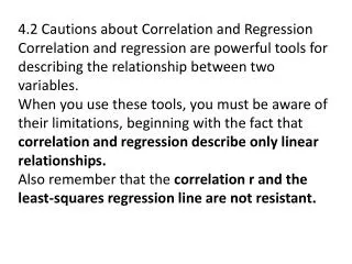
Model Assumptions & Problems • Linearity: Many relations are not perfectly linear, but can be well approximated by straight line over a range of X values • Extrapolation: While we can check validity of straight line relation within observed X levels, we cannot assume relationship continues outside this range • Influential Observations: Some data points (particularly ones with extreme X levels) can exert a large influence on the predicted equation.