Cavendish Experiment
Cavendish Experiment. Presented by Mark Reeher. Lab Partner: Jon Rosenfield For Physics 521. Presentation Overview. Historical Background Theory Experimental Setup and Methods Results Analysis of Results Uncertainties Conclusions. Brief Timeline of Gravitational Physics.

Cavendish Experiment
E N D
Presentation Transcript
Cavendish Experiment Presented by Mark Reeher Lab Partner: Jon Rosenfield For Physics 521
Presentation Overview • Historical Background • Theory • Experimental Setup and Methods • Results • Analysis of Results • Uncertainties • Conclusions
Brief Timeline of Gravitational Physics • 4th Century B.C: Aristotle – tendency of objects to be pulled to Earth • 1645: Ismael Bulliadus - inverse square relation • 1665: Sir Isaac Newton - • 1798: Henry Cavendish – calculation of Universal Gravitation Constant, G • Early 1900s: Einstein- • Inertia-gravitation equivalence • General relativity
Cavendish Experiment • John Michell – conception of experiment • Torsion Balance • Henry Cavendish – rebuilt balance and ran experiment in 1797-1798 • Basic Idea – directly measure Fg, find G • Found: G = 6.754 × 10⁻¹¹ m3kg-1s-2
Theory – Experimental Design • Large masses brought near small masses • Gravitational force movement in torsion balance • Study motion to determine Fg • With Fg, measure M, m, r • Newton’s gravitational equation • Result = calculated G
Top View Derivation - 1 Fβ Fα
Small Angle Approximation • For simplicity, we assume θ is very small • Torque dot product • Tan θ = θ • This assumption confirmed by finding the largest possible angle of setup • θmax = 0.03884 = 2.226º • ~0.05% difference between tan θ and θ
Experimental Setup Torsion balance enclosure Large masses Vacuum pump (oil) He-Ne laser Ametek plotter (converted)
Setup Diagram Laser Plotter
Setup Diagram So we need to keep in mind, the plotter reacts to 2θ
Fβ Fα Fα Fβ Setup Notes • Torsion enclosure pumped to ~100 mTorr • Data recorded automatically in Labview • Photodiode position vs time (4 s intervals) • Six total trials • 2 counter-clockwise (positive) torque • 2 clockwise (negative)torque • 2 no mass
Results (Our Measurements) • Given in lab manual • m = 0.019 kg • Mrod = 0.031 kg (square cross section) • L/2 = 15.24 cm • Distance measurements (in inches) • Dd (mirror-diode) = 45 1/32” • ω and θ are found from Matlab data 1 2 4 3
Analysis • Data from best fit: • General model: f(x) = a*exp(-x/b)*cos(c*x+d)+e • Coefficients (with 95% confidence bounds): a = 131 (130.4, 131.6) b = 1.029e+004 (1.006e+004, 1.051e+004) c = 0.007577 (0.007575, 0.007579) d = 0.004448 (0.0001244, 0.008771) e = 682.1 (681.9, 682.3) • Goodness of fit: SSE: 1000 R-square: 0.9986 Adjusted R-square: 0.9986 RMSE: 1.002
Analysis • I calculation • Κ calculation • Avg K = 2.60588 x 10⁻⁷+ 1.197 x 10⁻¹¹ kg m/s2
Analysis • ri calculation (m) • θ calculation • Avg eo from “NM” values: eo = 3.954” + 0.000177” • Define xi = eo - ei
Analysis • Now find θ from tan-1: • Finally… we find G (m3s-2): • Avg G = (3.89829 x 10⁻¹⁰+ 1.7129 x 10⁻¹¹)/M
Uncertainty • Total Uncertainty relation for G: 000000000000
Uncertainty • Each of the four variables also had combined uncertainty in their calculation • All type A aside from distance measurements • In a few cases, values were averaged:
Conclusions • M = 5.701 kg † • Gives us: • GCavendish = 6.754 × 10⁻¹¹ m3kg-1s-2 • GCODATA = 6.67428 × 10⁻¹¹ m3kg-1s-2 • Obvious setup interference • MEarth Accepted value = 5.97 x 1024 kg † conversation with Jose