Matrix sparsification (for rank and determinant computations)
280 likes | 475 Vues
Matrix sparsification (for rank and determinant computations). Raphael Yuster University of Haifa. Elimination, rank and determinants. Computing ranks and determinants of matrices are fundamental algebraic problems with numerous applications.

Matrix sparsification (for rank and determinant computations)
E N D
Presentation Transcript
Matrix sparsification(for rank and determinant computations) Raphael YusterUniversity of Haifa
Elimination, rank and determinants • Computing ranks and determinants of matrices are fundamental algebraic problems with numerous applications. • Both of these problems can be solved as by-products of Gaussian elimination (G.E.). • [Hopcroft and Bunch -1974]:G.E. of a matrix requires asymptotically the same number of operations as matrix multiplication. • The algebraic complexity of rank and determinant computation is O(nω) where ω < 2.38[Coppersmith and Winograd -1990].
Elimination, rank and determinants • Can we do better if the matrix is sparsehaving m << n2 non-zero entries? • [Yannakakis -1981]: G.E. is not likely to help. • If we allow randomness there are faster methods for computing the rank of sparse matrices . • [Wiedemann -1986] An O(n2+nm) Monte Carlo algorithm for a matrix over an arbitrary field. • [Eberly et al - 2007] An O(n3-1/(ω-1)) < O(n2.28) Las Vegas algorithm when m=(n).
Structured matrices • In some important cases that arise in various applications, the matrix possesses structural properties in addition to being sparse. • Let A be an n × nmatrix. The representing graphdenoted GA, has vertices {1,…,n} where:for i ≠ j we have an edge ijiffai,j≠ 0 or aj,i≠ 0. • GA is always an undirected simple graph.
Nested dissection • [Lipton, Rose, and Tarjan – 1979] Their seminal nested dissection method asserts that if A is- real symmetric positive definiteand- GA is represented by a -separator treethen G.E. on A can be performed in O(nω) time. • For < 1 better than general G.E. • Planar graphs and bounded genus graphs: = ½ [the separator tree constructed inO(n log n) time]. • For graphs with an excluded fixed minor: = ½ [ the separator tree can only be constructed inO(n1.5) time].
Nested dissection - limitations • Matrix needs to be: • Symmetric • Real • positive (semi) definite • The method does not apply to matrices over finite fields (not even GF(2)) nor to real non-symmetric matrices nor to symmetric non positive-semidefinite matrices. In other words: it is not general. • Our main result: we can overcome all of these limitations if we wish to compute ranks or absolute determinants. Thus making nested dissection a generalmethod for these tasks.
Matrix sparsification • Important tool used in the main result: Sparsification lemma • Let A be a square matrix of order n with m nonzero entries. Another square matrix B of order n+2t with t = O(m) is constructed in O(m) time so that: • det(B) = det(A) , • rank(B)=rank(A)+2t, • Each row and column of B have at most three non-zero entries.
Why is sparsification useful? • Usefulness of sparsification stems from the fact that • Constant powers of B are also sparse. • BDBT (where D is a diagonal matrix) is sparse. • This is not true for the original matrix A. • Over the reals we know that rank(BBT) = rank(B) = rank(A)+2t and also that det(BBT) = det(A)2. • Since BBT is symmetric, and positive semidefinite (over the reals), then the nested dissection method may apply if we can also guarantee that GBBT has a good separator tree (guaranteeing this, in general, is not an easy task).
Main result – for ranks Let A F n × n. If GA has bounded genus then rank(A) can be computed in O(nω/2) < O(n1.19) time. If GA excludes a fixed minor then rank(A) can be computed in O(n3ω/(3+ ω)) < O(n1.326) time. The algorithm is deterministic if F= Rand randomized if F is a finite field. Similar result obtained for absolute determinants of real matrices.
Sparsification algorithm • Assume that A is represented in a sparse form: Row lists Ri contain elements of the form (j , ai,j). • By using symbol 0* we can assume ai,j 0 aj,i 0. • At step t of the algorithm, the current matrix is denoted by Bt and its order is n+2t. Initially B0=A. • A single step constructs Bt +1 from Bt by increasing the number of rows and columns of Bt by 2 and by modifying constantly many entries of Bt. • The algorithm halts when each row list of Bt has at most three entries.
Sparsification algorithm – cont. • Thus, in the final matrix Bt we have that each row and column has at most 3 non-zero entries. • We make sure that:det(Bt+1) = det(Bt) and rank(Bt+1) = rank(Bt)+2. • Hence, in the end we will also havedet(Bt) = det(A) and rank(Bt) = rank(A)+2t. • How to do it:As long as there is a row with at least 4 nonzero entries, pick such row i and suppose bi,v 0 bi,u 0 .
Sparsification algorithm – cont. • Consider the principal block defined by {i , u , v}:
What happens in the representing graph? • Recall the vertex splitting trick : 8, -6 56 7 9, 0* … 13 8, -6 56 1, -1 1, -1 0 0 7 9, 0* … 13
A B C Separators At the top level:partition A,B,Cof the vertices of Gso that|C| = O(n)|A|, |B| < αnNo edges connect Aand B . Strong separator tree: recurse on A Cand on B C. Weak separator tree:recurse on Aand on B .
Finding separators Lipton-Tarjan (1979):Planar graphs have (O(n1/2), 2/3)-separators.Can be found in linear time. Alon-Seymour-Thomas (1990):H-minor free graphs have (O(n1/2), 2/3)-separators. Can be found in O(n1.5) time. Reed and Wood (2005):For any ν>0, there is an O(n1+ν)-time algorithm that finds (O(n(2ν)/3), 2/3)-separators ofH-minor free graphs.
Obstacle 1: preserving separators • Can we perform the (labeled) vertex splitting and guarantee that the modified representing graph still has a -separator tree ? • Easy for planar graphs and bounded genus graphs: just take the vertices u,vsplitted from vertex i to be on the same face. This preserves the genus. • Not so easy (actually, not true!) that splitting an H-minor free graph keeps it H-minor free. • [Y. and Zwick - 2007] vertex splitting can be performed while keeping the separation parameter (need to use weak separators). No “additional cost”.
Main technical lemma Suppose that (O(nβ),2/3)-separators of H-minor free graphs can be found in O(nγ)-time. If G is an H-minor free graph, then a vertex-split version G’ of G of bounded degree and an (O(nβ),2/3)-separator tree of G’ can be found in O(nγ) time.
Obstacle 2: separators of BDBT • We started with A for which GA has a -separator tree. • We used sparsification to obtain a matrix B withrank(B) = rank(A) + 2tfor which GB has bounded degree and also has a (weak) -separator tree. • We can compute, in linear time, BDBT where D is a chosen diagonal matrix. We do so because BDBT is always pivoting-free(analogue of positive definite). • But what about the graph GCof C= BDBT ?No problem! GC= (GB)2 (graph squaring of bounded degree graph): k-separator => O(k)-separator.
Obstacle 3: rank preservation of BDBT • Over the reals take D=Iand use rank(BBT)=rank(B) and we are done. • Over other fields (e.g. finite fields) this is not so: • If D = diag(x1,…,xn) we are OK over the generated ring: rank(BDBT)=rank(B) over F[x1,…,xn] . • Can’t just substitute the xi’s for random field elements and hope that w.h.p. the rank preserves! rank(B)=2 in GF(3) rank(BBT)=1 in GF(3)
Obstacle 3: cont. rank(B)=n/2in GF(p) Prob. (rank(BDBT))=n/2 is exponentially small • Solution: randomly replace the thexi’s with elements of a sufficiently large extension field. • If |F|=qsuffices to take extension field F ’ with qr elements where qr > 2n2 . Thusr = O(log n). • Constructing F ’ (generating irreducible polynomial ) takes O(r2 + r log q)time [Shoup – 1994].
Applications Maximum matching in bounded-genus graphs can be found in O(nω/2) < O(n1.19) time (rand.) Maximum matching in H-minor free graphs can be found in O(n3ω/(3+ω)) < O(n1.326) time (rand.) The number of maximum matchings in bounded-genus graphs can be computed deterministically in O(nω/2+1) < O(n2.19) time
4 1 6 3 2 5 Tutte’s matrix (Skew-symmetric symbolic adjacency matrix)
Tutte’s theorem Let G=(V,E) be a graph and let A be its Tutte matrix. Then, G has a perfect matching iff det A0. 1 2 4 3
Tutte’s theorem Let G=(V,E) be a graph and let A be its Tutte matrix. Then, G has a perfect matching iff det A0. Lovasz’s theorem Let G=(V,E) be a graph and let A be its Tutte matrix. Then, the rank of A is twice the size of a maximum matching in G.
Why randomization? It remains to show how to compute rank(A) (w.h.p.) in the claimed running time. By the Zippel / Schwarz polynomial identity testingmethod, we can replace the variables xij in Aswith random elements from {1,…,R} (where R ~ n2 suffices here) and w.h.p. the rank does not decrease. By paying a price of randomness, we remain with the problem of computing the rank of a matrix with small integer coefficients.