W in
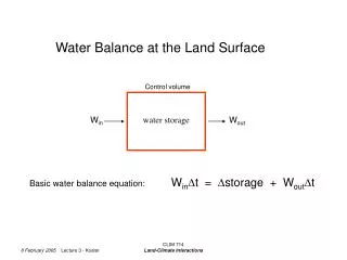
Control volume. W in. W out. water storage. W in D t = D storage + W out D t. Basic water balance equation:. Water Balance at the Land Surface. Water Balance for a Single Land Surface Slab, Without Snow (e.g., standard bucket model). Terms on LHS come from the climate model.

W in
E N D
Presentation Transcript
Control volume Win Wout water storage WinDt = Dstorage + WoutDt Basic water balance equation: Water Balance at the Land Surface CLIM 714 Land-Climate Interactions
Water Balance for a Single Land Surface Slab, Without Snow(e.g., standard bucket model) Terms on LHS come from the climate model. Strongly dependent on cloudiness, water vapor, etc. Terms on RHS come are determined by the land surface model. P = E + R + CwDw/Dt + miscellaneous P E R w where P = Precipitation E = Evaporation R = Runoff (effectively consisting of surface runoff and baseflow) Cw = Water holding capacity of surface slab Dw = Change in the degree of saturation of the surface slab Dt = time step length miscellaneous = conversion to plant sugars, human consumption, etc. CLIM 714 Land-Climate Interactions
DWc Dt P = Eint + Dc + P (snow) Esnow Wsnow M Usually, a combination of water balances is considered. For example: Water balance associated with canopy interception reservoir Eint = interception loss Dc = drainage through canopy (“throughfall”) DWc = change in canopy interception storage P Eint Wc Dc Water balance in a snowpack DWsnow Dt P = Esnow + M + Esnow = sublimation rate M = snowmelt DWsnow = change in snow amount (“infinite” capacity possible) CLIM 714 Land-Climate Interactions
Etr2 w1 Q12 water storage w2 Q23 w3 Water balance in a surface layer M + Dc = Ebs + Etr1 + Rs + Q12 + CW1DW1/Dt M+Dc Ebs + Etr1 Rs Water storage w1 Q12 Ebs = evaporation from bare soil Etr1 = evapotranspiration from layer 1 Q12 = water transport from layer 1 to layer 2 CW1 = water holding capacity of layer 1 DW1 = change in degree of saturation of layer 1 w2 w3 Water balance in a subsurface layer (e.g., 2nd layer down) Q12 = Q23 + Etr2 + CW2DW2/Dt Note: some models may include an additional, lateral subsurface runoff term Etr2 = evapotranspiration from layer 2 Q23 = water transport from layer 2 to layer 3 CW2 = water holding capacity of layer 2 DW2 = change in degree of saturation of layer 2 CLIM 714 Land-Climate Interactions
Etr-n Qn,n-1 water storage wn QD Water balance in the lowest layer Qn,n-1 = QD + Etr-n + CWnDWn/Dt Etr-n = evapotranspiration from layer n, if allowed QD = Drainage out of the soil column (baseflow) A model may compute all of these water balances, taking care to ensure consistency between connecting fluxes (in analogy with the energy balance calculation). P Eint Esnow P Dc Ebs Etr1 Etr2 Etr3 Rs M W1 Q12 W3 W2 Q23 QD CLIM 714 Land-Climate Interactions
Precipitation, P Getting the land surface hydrology right in a climate model is difficult largely because of the precipitation term. At least three aspects of precipitation must be handled accurately: a. Spatially-averaged precipitation amounts (along with annual means and seasonal totals) b. Subgrid distribution. c. Temporal variability and temporal correlations. Otherwise, even with a perfect land surface model, Perfect land surface model Garbage in Garbage out CLIM 714 Land-Climate Interactions
Accurate precipitation measurements are limited by availability of rain gauges…. Each box is ~250 km on a side … and by inherent inaccuracies in satellite-derived precipitation data How Good is the Estimated SSM/I Rain Rate Climatology Data? Over oceans, no “truth” data available for validations Nonsystematic error includes sampling and random Sampling error dominates F-13 and F-14 SSM/I, with similar sampling have similar error TMI has a slightly less, nonsystematic error Combining F-13 & F-14 almost satisfy the TRMM 1 mm/day and 10% for heavy rain GPM with 8 satellites will have 50% less error than combining F-13 & F-14 Technical notes for figure Figure compliments of Al Chang, NASA/GSFC CLIM 714 Land-Climate Interactions
Precipitation: subgrid variability (1) The bottom storm is more evenly distributed over the catchment than the top storm. Intuitively, the top storm will produce more runoff, even though the average storm depth over the catchment (E(Yo)) is smaller. Key points: -- Specifying subgrid variability of precipitation is critical to an accurate modeling of surface hydrology. -- A GCM is typically unable to specify the spatial structure of a given storm. The LSM typically has to “guess” it. From Fennessey, Eagleson, Qinliang, and Rodriguez-Iturbe, 1986. CLIM 714 Land-Climate Interactions
Precipitation: subgrid variability (2) Here, the two storms have similar spatial structure and total precipitation amounts. The locations of the storms, however, are different. If the top storm fell on more mountainous terrain than the bottom storm, the top storm might produce more runoff Key point: A GCM is typically unable to specify the subgrid location of a given storm. The LSM typically has to “guess” it. From Fennessey, Eagleson, Qinliang, and Rodriguez-Iturbe, 1986. CLIM 714 Land-Climate Interactions
GPM Mission Design • OBJECTIVES • Understand horizontal & vertical structure of rainfall, its macro- & micro-physical nature, & its associated latent heating • Train & calibrate retrieval algorithms for constellation radiometers • OBJECTIVES • Provide sufficient global sampling to significantly reduce uncertainties in short-term rainfall accumulations • Extend scientific and societal applications Core Constellation • Core Satellite • TRMM-like spacecraft (NASA) • H2-A rocket launch (NASDA) • Non-sun-synchronous orbit • ~ 65° inclination • ~400 km altitude • Dual frequency radar (NASDA) • K-Ka Bands (13.6-35 GHz) • ~ 4 km horizontal resolution • ~250 m vertical resolution • Multifrequency radiometer (NASA) • 10.7, 19, 22, 37, 85, (150/183 ?) GHz V&H • Constellation Satellites • Pre-existing operational-experimental & dedicated satellites with PMW radiometers • Revisit time • 3-hour goal at ~90% of time • Sun-synch & non-sun- synch orbits • 600-900 km altitudes • Precipitation Validation Sites for Error Characterization • Select/globally distributed ground validation “Supersites” (research quality radar, up looking radiometer-radar-profiler system, raingage-disdrometer network, & T-q soundings) • Dense & frequently reporting regional raingage networks • Precipitation Processing Center • Produces global precipitation products • Products defined by GPM partners CLIM 714 Land-Climate Interactions
time step 2 time step 3 time step 1 Case 1: No temporal correlation in storm position -- the storm is placed randomly with the grid cell at each time step. Case 2: Strong temporal correlation in storm position between time steps. Precipitation: temporal correlations Temporal correlations are very important -- but are largely ignored -- in GCM formulations that assume subgrid precipitation distributions. This is especially true when the time step for the land calculation is of the order of minutes. Why are temporal correlations important? Consider three consecutive time steps at a GCM land surface grid cell: Case 2 should produce, for example, stronger runoff. CLIM 714 Land-Climate Interactions
Throughfall Simplest approach: represent the interception reservoir as a bucket that gets filled during precipitation events and emptied during subsequent evaporation. Throughfall occurs when the precipitation water “spills over” the top of the bucket. Capacity of bucket is typically a function of leaf area index, a measure of how many leaves are present. This works, but because it ignores subgrid precipitation variability (e.g., fractional wetting), it is overly simple. CLIM 714 Land-Climate Interactions
Spatial precipitation variability and interception loss SiB’s approach (Seller’s et al, 1986) Precipitation assumed to fall according to some prescribed distribution Area above line is considered throughfall Capacity of reservoir Note: SiB allows some of the precipitation to fall to the ground without touching the canopy. Original water in reservoir CLIM 714 Land-Climate Interactions
Temporal precipitation variability and interception loss Mosaic LSM’s approach: CLIM 714 Land-Climate Interactions
Evaporation See notes from energy balance lecture. Note, though, locations of moisture sinks for bare soil evaporation and transpiration: Bare soil evaporation water is usually taken from the top soil layer. Transpiration water is usually taken from the soil layers that comprise the root zone. Different amounts may be taken from different layers depending on: -- layer thickness -- assumed root density profile e.g., transpiration water taken from these layers… but not this layer CLIM 714 Land-Climate Interactions
Runoff a. Overland flow: (i) flow generated over permanently saturated zones near a river channel system: “Dunne” runoff (ii) flow generated because precipitation rate exceeds the infiltration capacity of the soil (a function of soil permeability, soil water content, etc.): “Hortonian” runoff b. Interflow (rapid lateral subsurface flow through macropores and seepage zones in the soil c. Baseflow (return flow to stream system from groundwater) Runoff (streamflow) is affected by such things as: -- Spatial and temporal distributions of precipitation -- Evaporation sinks -- Infiltration characteristics of the soil -- Watershed topography -- Presence of lakes and reservoirs CLIM 714 Land-Climate Interactions
Modeling runoff: basin scale When variations in precipitation, topography, soil characteristics, etc., can be explicitly accounted for (as in so-called “spatially distributed” hydrological basin models), runoff can be predicted fairly accurately. The TOPMODEL approach uses the statistics of topography to characterize the spatial distribution of water table depth in a basin, with consequent impacts on runoff generation. simulated observed From Beven, K., “Spatially distributed modeling; conceptual approach to runoff prediction”, in Recent Advances in the Modeling of Hydrologic Systems, ed. By Bowles and O’Connell, p. 373-387, Kluwer Academeic Pub., 1991. CLIM 714 Land-Climate Interactions
Modeling runoff: GCM scale Surface runoff formulations in GCMs are generally very crude, for at least two reasons: (i) Developers of GCM precipitation schemes have focused on producing accurate precipitation means, not on producing accurate subgrid spatial and temporal variability. (ii) GCM land surface models generally represent the hydrological state of the grid cell with grid-cell average soil moistures -- the time evolution of subgrid soil moisture distributions is not monitored. At best, we can expect first-order success with these runoff formulations CLIM 714 Land-Climate Interactions
Controls in nature Framework of typical LSM SCALE: HUNDREDS OF KILOMETERS CLIM 714 Land-Climate Interactions
W1 W1max This part of the throughfall (above the line) runs off; the rest infiltrates throughfall distribution Depth =infiltration capacity * Dt Note that because of the inherent inconsistency between nature and the typical LSM’s soil layer framework, no “best” approach for modeling runoff exists. Current LSM approaches are “all over the place”. Typically, though, runoff is a function of the amount of moisture in the top soil layer. Bucket model: total runoff = P + M - E if this is positive and the bucket is full. total runoff = 0 otherwise. GISS Model II: total runoff = max( 0.5 P Dt, excess over capacity ). SiB: surface runoff = excess over infiltration capacity, assuming subgrid distribution of throughfall. Other approaches will be discussed later in the course. CLIM 714 Land-Climate Interactions
Where does GCM runoff go once it’s produced? It may “disappear” (i.e., since it eventually ends up in the ocean anyway, it may be no longer considered by the land model -- it may be effectively removed and forgotten), or it may be routed, using routing networks like this. The routed runoff can be compared to streamgauge measurements. CLIM 714 Land-Climate Interactions
(Implied) Global Annual River Discharge (kg/yr) Historical estimates of river discharge are all over the place -- more evidence of uncertainty in our estimates of the global water cycle. B0 P1 P2 P3 Legacy of estimates Schlosser and Houser, 2004 (submitted) CLIM 714 Land-Climate Interactions
Satellite measurements may provide valuable runoff data. (The methodology is still in its infancy.) Observations: River and Lake Stage Jehil Reservoir, Afghanistan TOPEX/POSEIDON-Radar Backscatter Jehil Reservoir1990 Jehil Reservoir1999 Jehil Reservoir2001 (dry) Jehil Reservoir1998 Application of satellite radar altimetry and imagery to drought investigation. C. Birkett/ESSIC CLIM 714 Land-Climate Interactions
Soil Moisture Transport, Baseflow First, some useful definitions: Porosity (n): The ratio of the volume of pore space in the soil to the total volume of the soil. When a soil with a porosity of 0.5 is completely dry, it is 50% rock by volume and 50% air by volume. Volumetric moisture content (q): The ratio of the volume of water in the soil to the total volume of soil. When the soil is fully saturated, q = n. Degree of saturation (w): The ratio of the volume of water in the soil to the volume of water at saturation. By definition, w= q /n. Pressure head (y): A measure of the degree to which the soil holds on to its water through tension forces. More specifically, y =p/rg, where r is the density of water, g is gravitational acceleration, and p is the fluid pressure. Elevation head (z): The height of soil element above an arbitrary baseline. Hydraulic head (h): The sum of the pressure head and the elevation head. Wilting point: The soil moisture content (measured either in degree of saturation or pressure head) at which plants can no longer draw the moisture from the soil. When modeling the root zone, this is often considered to be the lowest moisture content possible. Field capacity: The water content obtained when a saturated soil drains to the point where the surface tension on the soil particles balances the gravitational forces causing drainage. CLIM 714 Land-Climate Interactions
L h2 h1 Estimating water transport in the saturated zone (i.e., below water table) Darcy’s Law states that Q/A = flow per unit normal area = - K where K = hydraulic conductivity h = hydraulic head L = separation distance h2 - h1 L More generally, q = - K h q = specific discharge = Q/A Generalized Darcy’s Law: relates flow to gravitational and pressure forces. (Recall: h = y + z) CLIM 714 Land-Climate Interactions
krg K = m Hydraulic conductivity, K, is related to the soil’s specific permability: Where r is the fluid’s density and m is its dynamic viscosity. K is thus a function of soil and fluid properties. K varies tremendously with soil type. Small variations in soil type, say across a field site, could lead to orders of magnitude difference in the ability to transport moisture. From Freeze and Cherry CLIM 714 Land-Climate Interactions
y(w) = ysaturated w -b K(w) = Ksaturated w 2b+3 b = empirical coefficient Unsaturated zone equations (from Clapp and Hornberger) Moisture transport in the unsaturated zone (e.g., in the soil near the surface) can also be computed with Darcy’s law, if appropriate corrections are made to pressure head and hydraulic conductivity. qr = residual moisture “specific retention” Z If atmospheric pressure defined to be 0. qr Recall: q = ratio of water volume to soil volume, n = porosity Soil moisture profile capillary fringe p < 0 p = 0 q=n q p > 0 Water table Recall: w= degree of saturation, = q/n CLIM 714 Land-Climate Interactions
Soil parameter values used in GSWP, from Cosby m m/s CLIM 714 Land-Climate Interactions
Three things that complicate moisture transport in the unsaturated zone: 1. Extreme nonlinearity. b may have values between 4 and 10. If b=10, then K(q) = Ksaturated w23 2. Hysteresis Values of parameters not really a unique function of moisture state; they depend in part whether the soil has previously been wet or previously been dry -- whether the soil is wetting up or drying down. From Freeze and Cherry 3. Anisotropy. Hydraulic conductivity may vary with the direction of flow. For a given head gradient, flow in this direction may be easier than flow in this direction CLIM 714 Land-Climate Interactions
z z y h z GCM approaches to modeling subsurface flow Typically, -- Assume homogeneity of soil constant Ksat, ysat -- Ignore hysteresis -- Concentrate on vertical transports only -- Concentrate only on unsaturated zone and determination of moisture drainage to water table Discretization of Darcy’s law (e.g., SiB) Darcy’s law for vertical flow can be written: q = - K h qz = - K = - K (z + y) = - K ( + 1) CLIM 714 Land-Climate Interactions
w1 d1 surface layer w2 d2 root layer d3 w3 recharge layer One possible discretization of Darcy’s law (continued) Characterize the soil as stacked layers (d = thickness) Compute for each layer i: yi = ysat wi-b Ki = Ksat wi 2b+3 Compute flow from layer i to layer i+1: yi - yi+1 qz i,i+1 = K + 1 d K = “average” K across distance = (diKi + di+1Ki+1)/(di+di+1) d = effective depth for computing gradient = 0.5 (di+di+1) For drainage out the bottom of the soil column (QD), one might equate it to the hydraulic conductivity in the lowest layer. SiB, for example, goes beyond this by also applying a “mean slope angle” term, sin x: QD = K3 sin x CLIM 714 Land-Climate Interactions
It’s important to keep in mind that the different LSMs use very different discretizations of the soil column -- there is no one “right way” to do it. Discretizations and moisture transport paths for a wide variety of LSMs, as outlined by Wetzel and Chang (1996) CLIM 714 Land-Climate Interactions
Energy balance versus water balance Water balance: Implicit solution usually not necessary Results in updated water storage prognostics Energy balance: Implicit solution usually necessary Results in updated temperature prognostics How are the energy and water budgets connected? 1. Evaporation appears in both. 2. Albedo varies with soil moisture content. 3. Thermal conductivity varies with soil moisture content. 4. Thermal emissivity varies with soil moisture content. Question: Can we address how the energy and water budgets together control evaporation rates? CLIM 714 Land-Climate Interactions
Budyko’s analysis of energy and water controls over evaporation These assymptotes act as barriers to evaporation. CLIM 714 Land-Climate Interactions
CLIM 714 Land-Climate Interactions
CLIM 714 Land-Climate Interactions
The equation in fact characterizes the combined energy and water balance behavior of GCMs in general... CLIM 714 Land-Climate Interactions
… and can thus be used to explain, in part, differences in GCM behavior. Each letter corresponds to a different GCM CLIM 714 Land-Climate Interactions
What determines the shape of Budyko’s curve? If only annual means mattered, the observed curve should look like this: CLIM 714 Land-Climate Interactions
Seasonality, however, is important. CLIM 714 Land-Climate Interactions
Note that if these seasonal effects alone were considered, the observed curve would actually look like this: CLIM 714 Land-Climate Interactions
This effect can bring the curve in line with the observed curve. Note, though, that other effects also contribute to a region’s evaporation rate, including land surface properties and the temporal variation of precipitation. CLIM 714 Land-Climate Interactions
Budyko’s analysis: discussion 1. Annual precipitation and net radiation control, to first order, annual evaporation rates. 2. The spread of points around the Budyko curve is large, though, due to various additional factors: -- phasing of seasonal P and Rnet cycles -- interseasonal storage of moisture -- Other land surface or meteorological effects (vegetation type and resistance, topography, rainfall statistics, …) 3. Note also: -- Land surface processes affect the precipitation and net radiation forcing -- there’s not truly a clean separation between land and atmospheric effects. -- The land’s effects on hourly, daily and monthly evaporation are relatively much more important than they are on annual evaporation. CLIM 714 Land-Climate Interactions
Budyko’s equation for mean annual evaporation Modification for interannual variability: See Koster and Suarez, 1999 CLIM 714 Land-Climate Interactions
Rnet / lP E sE P sP CLIM 714 Land-Climate Interactions
sE sP Rnet / lP Equation works well when tested with GCM data: curve derived from Budyko equation CLIM 714 Land-Climate Interactions