Download
1 / 29
300 likes | 811 Vues
Models of Volatility Smiles I. Chapter 8: ADVANCED OPTION PRICING MODEL. Put-Call Parity Arguments. Put-call parity p +S 0 e -qT = c +K e –r T holds regardless of the assumptions made about the stock price distribution It follows that p mkt - p bs = c mkt - c bs. Implied Volatilities.

E N D
Models of Volatility Smiles I Chapter 8: ADVANCED OPTION PRICING MODEL
Put-Call Parity Arguments • Put-call parity p +S0e-qT = c +K e–r T holds regardless of the assumptions made about the stock price distribution • It follows that pmkt-pbs=cmkt-cbs
Implied Volatilities • When pbs=pmkt, it must be true that cbs=cmkt • It follows that the implied volatility calculated from a European call option should be the same as that calculated from a European put option when both have the same strike price and maturity • The same is approximately true of American options
Volatility Smile • A volatility smile shows the variation of the implied volatility with the strike price • The volatility smile should be the same whether calculated from call options or put options
Implied Volatility Strike Price The Volatility Smile for Foreign Currency Options
Implied Distribution for Foreign Currency Options • Both tails are heavier than the lognormal distribution • It is also “more peaked” than the lognormal distribution
The Volatility Smile for Equity Options Implied Volatility Strike Price
Implied Distribution for Equity Options • The left tail is heavier and the right tail is less heavy than the lognormal distribution
Other Volatility Smiles? What is the volatility smile if • True distribution has a less heavy left tail and heavier right tail • True distribution has both a less heavy left tail and a less heavy right tail
Possible Causes of Volatility Smile • Asset price exhibiting jumps rather than continuous change • Volatility for asset price being stochastic (One reason for a stochastic volatility in the case of equities is the relationship between volatility and leverage)
Volatility Term Structure • In addition to calculating a volatility smile, traders also calculate a volatility term structure • This shows the variation of implied volatility with the time to maturity of the option
Volatility Term Structure The volatility term structure tends to be downward sloping when volatility is high and upward sloping when it is low
Three Alternatives to Geometric Brownian Motion • Constant elasticity of variance (CEV) by Cox and Ross 1976 • Mixed Jump diffusion by Merton 1976 • Variance Gamma by Madan, Carr and Chang 1998
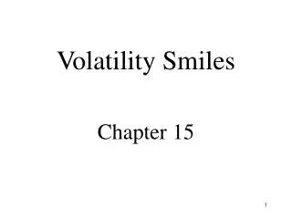
CEV Model • When a = 1 the model is Black-Scholes case • When a > 1 volatility rises as stock price rises • When a < 1 volatility falls as stock price rises • European option can be valued analytically in terms of the cumulative non-central chi-square distribution • Implied volatility imp = S-1.
simp a< 1 a > 1 CEV Models Implied Volatilities K/S
Distributional Implications • When a < 1 probability distribution similar to that observed for equities with heavy left tail and less heavy right tail. • When a > 1 probability distribution similar to that sometimes observed for options on futures with heavy right tail and a less heavy left tail.
CEV European Call and Put • When 0 < < 1, • When > 1,
CEV European Call and Put (Cont’d) • Where and 2(z,k,v) = noncentral chi-square distribution v = noncentrality parameter k = degrees of freedom less than z. • CEV model useful for valuing exotic equity models. Parameters of the model chosen to fit the prices of plain vanilla options by minimizing the sum of the squared differences between model prices and market prices.
Mixed Jump Diffusion Model • Merton produced a pricing formula when the stock price follows a diffusion process overlaid with random jumps • dp is the Poisson random jump • k is the expected size of the jump • ldt is the probability that a jump occurs in the next interval of length dt • dz is a Wiener process • dp and dz are independent • q dividend yields
Merton’s European Options • An important case is where the logarithm of the size of the percentage jump is normal. Merton shows the European price ’=(1+k) fn = Black-Scholes option price with dividend rate q. In fn , substitute 2+(ns2)/T for Variance rate and r-k+n/T for risk-free rate where s = standard deviation of the normal distribution of the logarithm of the size of percentage jump and = ln(1+k)
Jumps and the Smile • Gives rise to heavier left and right tails than Black-Scholes can be used for pricing currency options • Jumps have a big effect on the implied volatility of short term options • They have a much smaller effect on the implied volatility of long term options
The Variance-Gamma Model • A popular pure jump model • g is change over time T in a variable that follows a gamma process. This is a process where small jumps occur frequently and there are occasional large jumps • The probability density for g is of gamma distribution • (.) = gamma function
Understanding the Variance-Gamma Model • g defines the rate at which information arrives during time T (g is sometimes referred to as measuring economic time) • If g is large the the change in ln S has a relatively large mean and variance • If g is small relatively little information arrives and the change in ln S has a relatively small mean and variance
The Variance-Gamma Model (Cont’d) • Conditional on g, ln ST is normal. • The conditional mean = lnS0+(r-q)T+T+ g • The conditional standard deviation = • Its variance proportional to g • =(1/v) ln(1-v-2v/2) • There are 3 parameters • v, the variance rate of the gamma process • s2, the average variance rate of ln S per unit time • q, a parameter defining skewness
Skewness • When =0, lnST is symmetric • When <0, lnST is negatively skewed (as for equities) • When >0, lnST is positively skewed
Volatility Smile • The Variance-gamma model tends to produce U-shaped volatility smile. • Not necessarily symmetrical • Very pronounced for short maturities • Dies away for long maturities • Can be fitted to either equity or foreign currency plain vanilla option prices.
VG Option Pricing • Madan et al (1998) offers a semi-analytic European option valuation formula using the modified bessel function of the second kind and the degenerate hypergeometric function of two variables. • We can also calculate by Monte Carlo simulation.
VG Option Pricing (Cont’d) • The value g is generated by inverse gamma distribution function, i.e., g=Gamma-1(rn1;T/v, v) with random number rn1 from uniform distribution of zero mean and unit variance • The stock price ST is given by The value x is generated by inverse standard normal distribution function, i.e., x=N-1(rn2) • The European call price is • Therefore,