Volatility
Explore the definition, estimation, and implications of volatility, including VIX index, linear regression, heavy-tailed distributions, ARCH, GARCH models, and more in financial modeling.

Volatility
E N D
Presentation Transcript
Volatility Chapter 10
Motivation: • Until the early 80s econometrics had focused almost solely on modeling the means of series, i.e. their actual values. Recently however we have focused increasingly on the importance of volatility, its determinates and its effects on mean values.
Definition of Volatility • Suppose that Si is the value of a variable on day i. The volatility per day is the standard deviation of ln(Si /Si-1) • Normally days when markets are closed are ignored in volatility calculations • The volatility per year is times the daily volatility • Variance rate is the square of volatility
Standard Approach to Estimating Volatility • Define sn as the volatility per day between day n-1 and day n, as estimated at end of day n-1 • Define Si as the value of market variable at end of day i • Defineui= ln(Si/Si-1) 及以下公式
Simplifications Usually Made in Risk Management • Defineui as (Si−Si-1)/Si-1 • Assume that the mean value of ui is zero daily - short near 0 • Replace m-1 by m (high frequent) This gives
Implied Volatilities • Of the variables needed to price an option the one that cannot be observed directly is volatility • We can therefore imply volatilities from market prices and vice versa
VIX Index: A Measure of the Implied Volatility of the S&P 500
Linear Regression –the Workhorse of Financial Modeling • General form for the linear regression of Yt on • Variance of the error term is constant over time. This property is called conditional homoscedasticity
Distinction between the Conditional and Unconditional Variance • The unconditional variance is just the standard measure of the variance var(x) =E(x -E(x))2 • The conditional variance is the measure of our uncertainty about a variable given a model and an information set . cond var(x) =E(x-E(x| ))2 this is the true measure of uncertainty
Modeling conditional means and variances • If is N(0, 1), and Y = a + b, • then the mean is E(Y) = a • Var(Y ) = b2. • To model the conditional mean of Yt given • write Yt as the conditional mean plus white noise
Variation in the Conditional Variance • To allow a non-constant conditional variance in the model, multiply the white noise term by the conditional standard deviation. This product is added to the conditional mean as in the previous slide. • tmust be non-negative since it is a standard deviation
Stylized Facts of asset returns • Thick tails, they tend to be leptokurtic • Volatility clustering, Mandelbrot, ‘large changes tend to be followed by large changes of either sign’ • Leverage Effects, refers to the tendency for changes in stock prices to be negatively correlated with changes in volatility. • Forcastable events, volatility is high at regular times such as news announcements or other expected events, or even at certain times of day, e.g. less volatile in the early afternoon.
Heavy Tails • Daily exchange rate changes are not normally distributed • The distribution has heavier tails than the normal distribution • It is more peaked than the normal distribution • This means that small changes and large changes are more likely than the normal distribution would suggest • Many market variables have this property, known as excess kurtosis
References The classics: • Engle, R.F. (1982), Autoregressive Conditional Heteroskedasticity with Estimates of the Variance of U.K. • Bollerslev, T.P. (1986), Generalized Autoregresive Conditional Heteroscedasticity. Introduction/Reviews: • Bollerslev T., Engle R. F. and D. B. Nelson (1994), ARCH Models • Engle, R. F. (2001), GARCH 101: The Use of ARCH/GARCH Models in Applied Econometrics.
Weighting Scheme Instead of assigning equal weights to the observations when calculating volatility we can use different weights i for each observation
ARCH(q) ModelEngle(1982)Auto-Regressive Conditional Heteroscedasticity In an ARCH(q) model we also assign some weight to the long-run variance rate, VL:
Note: as we are dealing with a variance Even though the errors may be serially uncorrelated they are not independent, there will be volatility clustering and fat tails.
EWMA Model • In an exponentially weighted moving average model, the weights assigned to the u2 decline exponentially as we move back through time • This leads to (yesterday+
Attractions of EWMA • Relatively little data needs to be stored • We need only remember the current estimate of the variance rate and the most recent observation on the innovation to the market variable • Tracks volatility changes • RiskMetrics uses = 0.94 for daily volatility forecasting
GARCH(p,q) Bollerslev (1986) In empirical work with ARCH models high q is often required, a more parsimonious representation is the Generalised ARCH model VL= average of LT variance
GARCH (1,1) In GARCH (1,1) we assign some weight to the long-run average variance rate Since weights must sum to 1 + + =1
Example • Suppose • The long-run variance rate is 0.0002 so that the long-run volatility per day is 1.4%
Example continued • Suppose that the current estimate of the volatility is 1.6% per day and the most recent percentage change in the market variable is 1%. • The new variance rate is The new volatility is 1.53% per day
Independence vs. Zero Correlation • Independence implies zero correlation but not vice versa • GARCH processes are good examples • Dependence of the conditional variance on the past is the reason the process is not independent • Independence of the conditional mean on the past is the reason that the process is uncorrelated
Other Models • Many other GARCH models have been proposed • For example, we can design a GARCH models so that the weight given to i2 depends on whether i is positive or negative
Variance Targeting • One way of implementing GARCH(1,1) that increases stability is by using variance targeting • We set the long-run average volatility equal to the sample variance • Only two other parameters then have to be estimated
Maximum Likelihood Methods • All parameters in GARCH models are simply estimated by maximum likelihood using the same basic likelihood function, assuming normality • In maximum likelihood methods we choose parameters that maximize the likelihood of the observations occurring
Example 1 • We observe that a certain event happens one time in ten trials. What is our estimate of the proportion of the time, p, that it happens? • The probability of the outcome is • We maximize this to obtain a maximum likelihood estimate: p=0.1
Example 2 Estimate the variance of observations from a normal distribution with mean zero Observations are: The variance is denoted by The likelihood that ui is observed is given by the probability density function of the normal distribution:
The likelihood of n observations occurring in the order in which they are observed is:
Application to GARCH (1,1) We choose parameters that maximize
Forecasting and Persistence with GARCH(1,1) model Taking expectation at time t By repeated substitutions: As j→∞, the forecast reverts to the unconditional variance: ω/(1-α-β). When α+β=1, as in EWMA model, the expected future variance rate equals to today’s variance rate.

