The Coalescent and Measurably Evolving Populations
The Coalescent and Measurably Evolving Populations. Alexei Drummond Department of Computer Science University of Auckland, NZ. Overview. Introduction to the Coalescent Hepatitis C in Egypt An example using the coalescent Measurably evolving populations
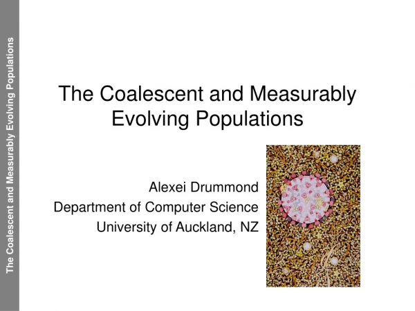

The Coalescent and Measurably Evolving Populations
E N D
Presentation Transcript
The Coalescent and Measurably Evolving Populations Alexei Drummond Department of Computer Science University of Auckland, NZ
Overview • Introduction to the Coalescent • Hepatitis C in Egypt • An example using the coalescent • Measurably evolving populations • HIV-1 evolution within and among hosts • An example using MEP concepts • Summary + Conclusions
The coalescent • The coalescent is a model of the ancestral relationships of a small sample of individuals taken from a large background population. • The coalescent describes a probability distribution on ancestral genealogies (trees) given a population history. • Therefore the coalescent can convert information from ancestral genealogies into information about population history and vice versa. • The coalescent is a model of ancestral genealogies, not sequences, and its simplest form assumes neutral evolution.
The history of coalescent theory • 1930-40s: Genealogical arguments well known to Wright & Fisher • 1964: Crow & Kimura: Infinite Allele Model • 1966: (Hubby & Lewontin) & (Harris) make first surveys of population allele variation by protein electrophoresis • 1968: Motoo Kimura proposes neutral explanation of molecular evolution & population variation. So do King & Jukes • 1971: Kimura & Ohta proposes infinite sites model. • 1975: Watterson makes explicit use of “The Coalescent” • 1982: Kingman introduces “The Coalescent”. • 1983: Hudson introduces “The Coalescent with Recombination” • 1983: Kreitman publishes first major population sequences. • 1987: Cann et al. traces human origin and migrations with mitochondrial DNA.
The history of coalescent theory • 1988: Hughes & Nei: Genes with positive Darwinian Selection. • 1989-90: Kaplan, Hudson, Takahata and others: Selection regimes with coalescent structure (MHC, Incompatibility alleles). • 1991: MacDonald & Kreitman: Data with surplus of replacement interspecific substitutions. • 1994-95: Griffiths-Tavaré + Kuhner-Yamoto-Felsenstein introduces sampling techniques to estimate parameters in population models. • 1997-98: Krone-Neuhauser introduces Ancestral Selection Graph • 1999: Wiuf & Donnelly uses coalescent theory to estimate age of disease allele • 2000: Wiuf et al. introduces gene conversion into coalescent. • 2000-: A flood of SNP data & haplotypes are on their way.
Population processes COALESCENT THEORY Genealogy
Coalescent inference Randomly sample individuals from population Obtain gene sequences from sampled individuals Reconstruct tree / trees from sequences Infer coalescent results directly from sequences Infer coalescent results from tree / trees
Demographic History • Change in population size through time • Applications include • Estimating history of human populations • Conservation biology • Reconstructing infectious disease epidemics • Investigating viral dynamics within hosts
Grand parents Parents Now Idealized Wright-Fisher populations Diploid Haploid
Random mating in an ideal population • A constant population size of N individuals • Each individual in the new generation “chooses” its parent from the previous generation at random
Genetic drift: extinction and ancestry If you trace the ancestry of a sample of individuals back in time you inevitably reach a single most recent common ancestor. If you pick a random individual and trace their descendents forward in time, all the descendents of that individual will with high probability eventually die out.
Past Present A sample genealogy from an idealized Wright-Fisher population Past A sample genealogy of 3 sequences from a population (N =10). Discrete Generations Present
The coalescent: distributions and expectations on a sample genealogy Past Present
The coalescent: probability density distribution Past Present The genealogy is an edge graph Eg and a vector of times t. Kingman (1982a,b)
The coalescent: estimating population size from a sample genealogy Past Present Felsenstein (1992)
The coalescent: estimating population size confidence limits via ML The confidence intervals are calculated from the curvature of the likelihood. For a single parameter model the 95% confidence limits are defined by the points where the log-likelihood drops 1.92 log-units below the maximum log-likelihood. Maximum likelihood can be used to estimate population size by choosing a population size that maximizes the probability of the observed coalescent waiting times.
The Coalescent The coalescent: shapes of gene genealogies Exponential growth Constant size The coalescent can be used to convert coalescent times into knowledge about population size and its change though time.
The Coalescent Constant population size: N(t)=N0 smallN0 large N0 TIME
The Coalescent Coalescent and serial samples Exponential growth Constant population
The Coalescent Uncertainty in Genealogies How similar are these two trees? Both of them are plausible given the data. We can use MCMC to get the average result over all plausible trees,
The Coalescent Coalescent Summary • The coalescent provides a theory of how population size is related to the distribution of coalescent events in a tree. • Big populations have old trees • Exponentially growing populations have star-like trees • Given a genealogy the most likely population size can be estimated. • MCMC can be used to get a distribution of trees from which a distribution of population sizes can be estimated.
MCMC Markov chain Monte Carlo (MCMC) • Imagine you would like to estimate two parameters (,) from some data (D). • You want to find values of and that have high probability given the data: p(,|D) • Say you have a likelihood function of the form: Pr{D| ,} • Bayes rule tells us that: • p(,|D) = Pr{D| ,}p(,) / Pr{D} • So that p(,|D) Pr{D| ,}p(,)
MCMC Markov chain Monte Carlo (MCMC) • p(,|D) is called the posterior probability (density) of , given D • In an ideal world we want to know the posterior density for all possible values of ,. • Then we could pick a “credible region” in two dimensions that contained values of , that account for the majority of the posterior probability mass. • This credible region would serve as an estimate that includes incorporates our uncertainty and this credible set could be used to address hypotheses like: is greater than x. • In reality we have to make due with a “sample” of the posterior - so that we evaluate p(,|D) for a finite number (say 10,000,000) pairs of ,. • So which pairs should we choose?
MCMC Markov chain Monte Carlo (MCMC) • Lets construct a random walk in 2-dimensional space • In each step of the random walk we propose to make an (unbiased) small jump from our current position (,) to a new position (’,’) • If p(’,’|D) > p(,|D) then we make the proposed jump • However, if p(’,’|D) < p(,|D), then we make the proposed jump with probability = p(’,’|D) / p(,|D), otherwise we stay where we are. • It can be shown (trust me!) that if you proceed in this fashion for an infinite time then the equilibrium distribution of this random walk will be p(,|D)! • That is, the random walk will visit a particular region [0, 1] x [0, 1] of the state space this often:
MCMC Markov chain Monte Carlo (MCMC)
Population genetics of Hepatitis C in Egypt Hepatitis C Virus (HCV) • Identified in 1989 • 9.6kb single-stranded RNA genome • Polyprotein cleaved by proteases • No efficient tissue culture system
Population genetics of Hepatitis C in Egypt How important is HCV? • 170m+ infected • ~80% infections are chronic • Liver cirrhosis & cancer risk • 10,000 deaths per year in USA • No protective immunity?
Population genetics of Hepatitis C in Egypt HCV Transmission Percutaneous exposure to infected blood • Blood transfusion / blood products • Injecting & nasal drug use • Sexual & vertical transmission • Unsafe injections • Unidentified routes
Population genetics of Hepatitis C in Egypt Estimating demographic history of HCV using the coalescent • Egyptian HCV gene sequences • n=61 • E1 gene, 411bp • All sequence contemporaneous • Egypt has highest prevalence of HCV worldwide (10-20%) • But low prevalence in neighbouring states • Why is Egypt so seriously affected? • Parenteral antischistosomal therapy (PAT)
Population genetics of Hepatitis C in Egypt Demographic model • The coalescent can be extended to model deterministically varying populations. • The model we used was a const-exp-const model. • A Bayesian MCMC method was developed to sample the gene genealogy, the substitution model and demographic function simultaneously.
Population genetics of Hepatitis C in Egypt Estimated demographic history Based on a single tree Averaged over all trees
Population genetics of Hepatitis C in Egypt Parameter estimates
Population genetics of Hepatitis C in Egypt Uncertainty in parameter estimates Demographic parameters Mutational parameters Growth rate of the growth phase Grey box is the prior Rates at different codon positions, All significantly different
Population genetics of Hepatitis C in Egypt Full Bayesian Estimation • Marginalized over uncertainty in genealogy and mutational processes • Yellow band represents the region over which PAT was employed in Egypt
Measurably evolving populations Present time point (n = 5) Earlier time point (n = 5) Measurably evolving populations (MEPs) • MEP pathogens: • HIV • Hepatitis C • Influenza A • MEPs from ancient DNA • Bison • Brown Bears • Adelie penguins • Anything cold and numerous • Even over short periods (less than a year) HIV sequences can exhibit measurable evolutionary change • Time-structure can not be ignored in our models
Measurably evolving populations Time structure in samples time Contemporary sample no time structure Serial sample with time structure 1980 1990 2000
Measurably evolving populations Molecular evolution and population genetics of MEPs • Given sequence data that is time-structured estimate true values of: • substitution parameters • Overall substitution rate and relative rates of different substitutions • population history: N(t) • Ancestral genealogy • Topology • Coalescent times m Ne time A B C D E
AC b4 AA b1 b3 b2 GA b5 GC Molecular evolutionary model: Felsenstein’s likelihood (1981) The probability of the sequence alignment, can be efficiently calculated given a tree and branch lengths (T), and a probabilistic model of mutation represented by an instantaneous rate matrix (Q). In phylogenetics, branch lengths are usually unconstrained.
Combining the coalescent with Felsenstein’s likelihood AC b4 t2 AA The “molecular clock” constraint b1 b3 t3 b2 GA b5 t4 AA GA AC GC GC 2n–3 branch lengths n–1 waiting times The joint posterior probability of the population history (N), the genealogy (g) and the mutation matrix (Q) are estimated using Markov chain Monte Carlo (Drummond et al, Genetics, 2002)
Measurably evolving populations 1 Z Full Bayesian Model Probability of what we don’t know given what we do know. Likelihood function other priors P(g, , Ne, Q | D) P(D | g, , Q)fG(g | Ne) f()fN(Ne)fQ(Q) = Unknown normalizing constant coalescent prior Q = substitution parameters Ne = population parameters g = tree = overall substitution rate In the software package BEAST, MCMC integration can be used to provide a chain of samples from this density.
Measurably evolving populations Pt.9 Pt.2 HIV1U35926 Pt.7 Patient #6 from Wolinsky et al. HIVU95460 Pt.5 HIV1U36148 Pt.6 HIV1U36073 HIV1U36015 HIV1U35980 Pt.8 Pt.3 Pt.1 10% HIV-1 (env) evolution in nine infected individuals Shankarappa et al (1999)
Measurably evolving populations 10% Viral Divergence 8% 6% 4% 2% 0 2 4 6 8 10 Years Post Seroconversion Molecular clock: HIV-1 (env) evolution in 9 individuals Shankarappa et al (1999)
Measurably evolving populations MEP Summary • Most RNA viruses, including HCV and HIV are measurably evolving • Most vertebrate populations that have well-preserved recent fossil records are MEPs. • If sequence data comes from different times the time-structure can’t be ignored • Time structure permits the direct estimation of: • substitution rate • Concerted changes in substitution rate • coalescent times in calendar units • Demographic function N(t) in calendar units
Intermission My brain is fried!
Population genetics of HIV What is HIV? • HIV is a retrovirus. • Within infected individuals HIV exhibits extremely high genetic variability due to: • Error-prone reverse transcriptase (RT) that converts RNA to DNA (error rate is about one mutation per genome per replication cycle). • DNA-dependent polymerase also error-prone • High turnover of virus within infected individual throughout infection.
Population genetics of HIV Number of sequences obtained per sample 11 22 20 8 20 20 20 10 8 20 9 20 22 12 20 30 40 51 61 68 73 80 85 91 103 126 Time in months (post seroconversion) Patient 2 (Shankarappa et al, 1999) 0 0 • 210 sequences collected over a period of 9.5 years • 660 nucleotides from env: C2-V5 region • Effective population size and mutation rate were co-estimated using Bayesian MCMC.
Population genetics of HIV A tree sampled from the posterior distribution ‘Ladder-like’ appearance Lineage A Lineage B
Population genetics of HIV Estimated substitution rate • Patient 2: • 0.77–1.0% per year • BUT…. Long term rates in HIV • Korber et al: • 0.24% (0.18-0.28%) per year • Only 1/4 of the intrapatient rate
Measurably evolving populations Bayesian MCMC of Shankarappa data
Population genetics of HIV Intra- and inter- patient rate estimates (C2V3 envelope) p1 - p11 C A B