Download
1 / 9

E N D
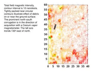
Total field magnetic intensity, contour interval is 10 nanotesla. Tightly packed near circular contours illustrate effect of debris on or near the ground surface. The prominent north-south corrugation is in the direction of acquisition with a Cesium vapor magnetometer. The tall axis trends 130o east of north.
Decorrugated total field intensity with regional field of about 54,000 nT removed • Decorrugation steps Urquhart (1988): • Apply a low pass filter to separate the grid of data into its short and long wavelength components in the acquisition direction. • the resulting long wavelength component of the grid is long-wavelength filtered (low pass) in the direction perpendicular to the acquisition direction. This removes short wavelength components, perpendicular to acquisition, that result from varying heights of the sensor. • Add the smoothed results from step two to the short wavelength components isolated in step one. Urquhart, T., 1988. Decorrugation of enhanced magnetic field maps. 58th Annual International Meeting, SEG, Expanded Abstracts, 371–372
Original TMI on left, decorrugated TMI on right. Contour interval 5 nanotesla.
Decorrugated TMI on left, that part of the observed field removed on right.
Enhanced signals from causative sources on or near the surface. Left: analytic signal of the total magnetic intensity. Right: synthetic vertical gradient calculated by differencing the total field intensity with an upward continuation of 0.2 meters; the zero contour is suppressed for clarity.
Radially averaged power spectrum of the total field magnetic intensity. Lines fit to symbols indicate separation of two equivalent layers as basis for matched bandpass filters Decorrugated TMI.
Radially averaged power spectrum of the total field magnetic intensity. Lines fit to symbols indicate separation of two equivalent layers as basis for matched bandpass filters. Matched bandpass filters in the spatial frequency domain. Triangles show bandpass for long wavelength signal, diamonds indicate bandpass for short wavelength signals.
Total field magnetic intensity separated into two equivalent layers. Left: deeper layer resulting from applying the long wavelength bandpass filter to total field intensity; contours are 2 nT to illustrate separation of signals from shallow dipolar sources. Right: anomalies from on or near surface sources; the zero contour is removed for clarity. The sum of these two maps equals the original decorrugated data.
Original (unfiltered) TMI Decorrugated lower equivalent layer