CMPS 3120: Computational Geometry Spring 2013

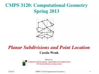
1. CMPS 3120: Computational GeometrySpring 2013 p Planar Subdivisions and Point Location CarolaWenk Based on:Computational Geometry: Algorithms and Applicationsand David Mount’s lecture notes CMPS 3120 Computational Geometry

2. Planar Subdivision • Let G=(V,E) be an undirected graph. • G is planar if it can be embedded in the plane without edge crossings. planar K5, not planar K3,3, not planar • A planar embedding (=drawing) of a planar graph G induces a planar subdivision consisting of vertices, edges, and faces. CMPS 3120 Computational Geometry

3. Doubly-Connected Edge List • The doubly-connected edge list (DCEL) is a popular data structure to store the geometric and topological information of a planar subdivision. • It contains records for each face, edge, vertex • (Each record might also store additional application-dependent attribute information.) • It should enable us to perform basic operations needed in algorithms, such as walk around a face, or walk from one face to a neighboring face • The DCEL consists of: • For each vertex v, its coordinates are stored in Coordinates(v) and a pointer IncidentEdge(v) to a half-edge that has v as it origin. • Two oriented half-edges per edge, one in each direction. These are called twins. Each of them has an origin and a destination. Each half-edge e stores a pointer Origin(e), a pointer Twin(e), a pointer IncidentFace(e) to the face that it bounds, and pointers Next (e) and Prev(e) to the next and previous half-edge on the boundary of IncidentFace(e). • For each face f, OuterComponent(f) is a pointer to some half-edge on its outer boundary (null for unbounded faces). It also stores a list InnerComponents(f) which contains for each hole in the face a pointer to some half-edge on the boundary of the hole. CMPS 3120 Computational Geometry

4. Complexity of a Planar Subdivision • The complexity of a planar subdivision is: #vertices + #edges + #faces = nv + ne + nf • Euler’s formula for planar graphs: • nv - ne + nf≥ 2 • ne ≤ 3nv – 6 2) follows from 1): Count edges. Every face is bounded by ≥ 3 edges. Every edge bounds ≤ 2 faces.  3nf ≤ 2ne  nf ≤ 2/3ne  2≤ nv - ne + nf≤ nv - ne + 2/3 ne = nv – 1/3 ne  2 ≤ nv – 1/3 ne • So, the complexity of a planar subdivision is linear in the number of vertices, so, O(nv). CMPS 3120 Computational Geometry

5. Point Location p • Point location task: Preprocess a planar subdivision to efficiently answer point-location queries of the type: Given a pointp=(px,py), find the face it lies in. • Important metrics: • Time complexity for preprocessing = time to construct the data structure • Space needs to store the data structure • Time complexity for querying the data structure CMPS 3120 Computational Geometry

6. Slab Method • Slab method: Draw a vertical line through each vertex. This decomposes the plane into slabs. p p p • In each slab, the vertical order of the line segments remains constant. • If we know in which slab p lies, we can perform binary search, using the sorted order of the segments in the slab. • Find slab that contains p by binary search on xamong slab boundaries. • A second binary search in slab determines the face containing p. • Search complexity O(log n), but space complexity (n2) . lower bound? CMPS 3120 Computational Geometry

7. Kirkpatrick’s Algorithm b • Needs a triangulation as input. • Can convert a planar subdivision with n vertices into a triangulation: • Triangulate each face, keep same label as original face. • If the outer face is not a triangle: • Compute the convex hull of the subdivision. • Triangulate pockets between the subdivision and the convex hull. • Add a large triangle (new verticesa,b,c) around the convex hull, and triangulate the space in-between. p a c • The size of the triangulated planar subdivision is still O(n), by Euler’s formula. • The conversion can be done in O(n log n) time. • Given p, if we find a triangle containing p we also know the (label of) the original subdivision face containing p. CMPS 3120 Computational Geometry

8. Kirkpatrick’s Hierarchy • Compute a sequence T0, T1, …, Tkof increasingly coarser triangulations such that the last one has constant complexity. • The sequence T0, T1, …, Tkshould have the following properties: • T0is the input triangulation, Tkis the outer triangle • k O(log n) • Each triangle in Ti+1overlaps O(1) triangles in Ti • How to build such a sequence? • Need to delete vertices from Ti . • Vertex deletion creates holes, which needto be re-triangulated. • How do we go from T0of size O(n) toTkof size O(1) in k=O(log n) steps? • In each step, delete a constant fractionof vertices from Ti. • We also need to ensure that each new triangle in Ti+1 overlaps with only O(1) triangles in Ti. CMPS 3120 Computational Geometry

9. Vertex Deletion and Independent Sets When creating Ti+1 from Ti , delete vertices from Ti that have the following properties: • Constant degree:Each vertex v to be deleted has O(1) degree in the graph Ti . • If v has degree d, the resulting hole can be re-triangulated with d-2 triangles • Each new triangle in Ti+1 overlaps at most d original triangles in Ti • Independent sets:No two deleted vertices are adjacent. • Each hole can be re-triangulated independently. CMPS 3120 Computational Geometry

10. Independent Set Lemma Lemma: Every planar graph on n vertices contains an independent vertex set of size n/18 in which each vertex has degree at most 8. Such a set can be computed in O(n) time. Use this lemma to construct Kirkpatrick’s hierarchy: • Start with T0, and select an independent set Sof size n/18 with maximum degree 8. [Never pick the outer triangle vertices a, b, c.] • Remove vertices of S, and re-triangulate holes. • The resulting triangulation, T1, has at most 17/18n vertices. • Repeat the process to build the hierarchy, until Tk equals the outer triangle with vertices a, b, c. • The depth of the hierarchy is k = log18/17 n b a c CMPS 3120 Computational Geometry

11. Hierarchy Example Use this lemma to construct Kirkpatrick’s hierarchy: • Start with T0, and select an independent set Sof size n/18 with maximum degree 8. [Never pick the outer triangle vertices a, b, c.] • Remove vertices of S, and re-triangulate holes. • The resulting triangulation, T1, has at most 17/18n vertices. • Repeat the process to build the hierarchy, until Tk equals the outer triangle with vertices a, b, c. • The depth of the hierarchy isk = log18/17 n CMPS 3120 Computational Geometry

12. Hierarchy Data Structure Store the hierarchy as a DAG: • The root is Tk. • Nodes in each level correspond to triangles Ti . • Each node for a triangle in Ti+1 stores pointers to all triangles of Ti that it overlaps. How to locate point p in the DAG: • Start at the root. If p is outside of Tkthen p is in exterior face; done. • Else, set  to be the triangle at the current level that contains p. • Check each of the at most 6 triangles of Tk-1 that overlap with , whether they contain p. Update  and descend in the hierarchy until reaching T0 . • Output  . p CMPS 3120 Computational Geometry

13. Analysis • Query time is O(log n): There are O(log n) levels and it takes constant time to move between levels. • Space complexity is O(n): • Sum up sizes of all triangulations in hierarchy. • Because of Euler’s formula, it suffices to sum up the number of vertices. • Total number of vertices:n + 17/18 n + (17/18)2 n + (17/18)3 n + … ≤ 1/(1-17/18) n = 18 n • Preprocessing time is O(n log n): • Triangulating the subdivision takes O(n log n) time. • The time to build the DAG is proportional to its size. p CMPS 3120 Computational Geometry 13

14. Independent Set Lemma Lemma: Every planar graph on n vertices contains an independent vertex set of size n/18 in which each vertex has degree at most 8. Such a set can be computed in O(n) time. • Proof: • Algorithm to construct independent set: • Mark all vertices of degree ≥ 9 • While there is an unmarked vertex • Let v be an unmarked vertex • Add v to the independent set • Mark v and all its neighbors • Can be implemented in O(n) time: Keep list of unmarked vertices, and store the triangulation in a data structure that allows finding neighbors in O(1) time. v CMPS 3120 Computational Geometry

15. Independent Set Lemma • Still need to prove existence of large independent set. • Euler’s formula for a triangulated planar graph on n vertices:#edges = 3n – 6 • Sum over vertex degrees:deg(v) = 2 #edges = 6n – 12 < 6n • Claim: At least n/2 vertices have degree ≤ 8.Proof: By contradiction. So, suppose otherwise. n/2 vertices have degree ≥ 9. The remaining have degree ≥ 3.  The sum of the degrees is ≥ 9 n/2 + 3 n/2 = 6n. Contradiction. • In the beginning of the algorithm, at least n/2 nodes are unmarked. Each picked vertex v marks ≤ 8 other vertices, so including itself 9. • Therefore, the while loop can be repeated at least n/18 times. • This shows that there is an independent set of size at least n/18 in which each node has degree ≤ 8. v CMPS 3120 Computational Geometry

16. Summing Up • Kirkpatrick’s point location data structure needs O(n log n) preprocessing time, O(n) space, and has O(log n) query time. • It involves high constant factors though. • Next we will discuss a randomized point location scheme (based on trapezoidal maps) which is more efficient in practice. CMPS 3120 Computational Geometry

17. Trapezoidal map • Input: Set S={s1,…,sn} of non-intersecting line segments. • Query: Given point p, report the segment directly above p. • Create trapezoidal map by shooting two rays vertically (up and down) from each vertex until a segment is hit. [Assume no segment is vertical.] • Trapezoidal map = rays + segments • Enclose S into bounding box to avoidinfinite rays. • All faces in subdivision are trapezoids,with vertical sides. • The trapezoidal map has at most6n+4 vertices and 3n+1 trapezoids: • Each vertex shoots two rays, so, 2n(1+2)vertices, plus 4 for the bounding box. • Count trapezoids by vertex that creates itsleft boundary segment: Corner of box forone trapezoid, right segment endpoint forone trapezoid, left segment endpoint forat most two trapezoids.  3n+1 CMPS 3120 Computational Geometry

18. Construction • Randomized incremental construction • Start with outer box which is a single trapezoid. Then add one segment si at a time, in random order. si CMPS 3120 Computational Geometry

19. Construction • Let Si={s1,…, si}, and let Ti be the trapezoidal map for Si. • Add si to Ti-1. • Find trapezoid containing left endpoint of si. [Point location; do later] • Thread si through Ti-1, by walking through it and identifying trapezoids that are cut. • “Fix trapezoids up” by shooting rays from left and right endpoint of si and trim earlier rays that are cut by si. si CMPS 3120 Computational Geometry

20. Analysis • Observation: The final trapezoidal map Ti does not depend on the order in which the segments were inserted. • Lemma: Ignoring the time spent for point location, the insertion of si takes O(ki) time, where ki is the number of newly created trapezoids. • Proof: • Let k be the number of ray shots interrupted by si. • Each endpoint of si shoots two rays ki=k+4 rays need to be processed • If k=0, we get 4 new trapezoids. • Create a new trapezoid for each interrupted ray shot; takes O(1) time with DCEL si si CMPS 3120 Computational Geometry

21. Analysis n/2+1 n/2+2 n 1 n/2 2 3 • Insert segments in random order: • P = {all possible permutations/orders of segments}; |P| = n! for n segments • ki = ki(p) for some random order pP • We will show that E(ki)=O(1) •  Expected runtimeE(T) = E(i=1ki)=i=1E(ki)= O(i=11)= O(n) n n n linearity of expectation CMPS 3120 Computational Geometry

22. Analysis • Theorem: E(ki)=O(1), where ki is the number of newly created trapezoids created upon insertion of si, and the expectation is taken over all segment permutations of Si={s1,…, si}. • Proof: • Ti does not depend on the order in which segments s1,…, siwere added. • Of s1,…, si, what is the probability that a particular segment s was added last? • 1/i • We want to compute the number of trapezoids that would have been created if s was added last. CMPS 3120 Computational Geometry

23. Analysis • Random variable ki(s)=#trapezoids added when s was inserted last Si. • ki(s)= • E(ki)= CMPS 3120 Computational Geometry

24. Analysis • Random variable ki(s)=#trapezoids added when s was inserted last Si. • ki(s)= • E(ki)= • = • How many segments does D depend on? At most 4. • Also, Ti has O(i) trapezoids (by Euler’s formula). • E(ki)== CMPS 3120 Computational Geometry

25. Point Location • Build a point location data structure; a DAG, similar to Kirkpatrick’s • DAG has two types of internal nodes: • x-node (circle): contains the x-coordinate of a segment endpoint. • y-node (hexagon): pointer to a segment • The DAG has one leaf for each trapezoid. • Children of x-node: Space to the left and right of x-coordinate • Children of y-node: Space above and below the segment • y-node is only searched when the query’s x-coordinate is within the segment’s span. •  Encodes trapezoidal decomposition and enables point location during construction. CMPS 3120 Computational Geometry

26. Construction • Incremental construction during trapezoidal map construction. • When a segment s is added, modify the DAG. • Some leaves will be replaced by new subtrees. • Each old trapezoid will overlap O(1) new trapezoids. • Each trapezoid appears exactly once as a leaf. • Changes are highly local. • If s passes entirely through trapezoid t, then t is replaced with two new trapezoids t’and t’’ . • Add new y-node as parent of t’ and t’’ , in order to facilitate search later. • If an endpoint of s lies in trapezoid t, then add an x-node to decide left/right and a y-node for the segment. CMPS 3120 Computational Geometry

27. Inserting a Segment • Insert segment s3. • q3 s3 • p3 • q3 s3 • p3 CMPS 3120 Computational Geometry

28. Analysis • Space: Expected O(n) • Size of data structure = number of trapezoids = O(n) in expectation, since an expected O(1) trapezoids are created during segment insertion • Query time: Expected O(log n) • Construction time: Expected O(n log n) follows from query time • Proof that the query time is expected O(log n): • Fix a query point Q. • Consider how Q moves through the trapezoidal map as it is being constructed as new segments are inserted. • Search complexity = number of trapezoids encountered by Q s3 s3 CMPS 3120 Computational Geometry

29. Query Time • Let Dibe the trapezoid containing Q after the insertion of ith segment. • If Di=Di-1then the insertion does not affect Q’s trapezoid (E.g., QB). • If Di≠Di-1then the insertion deleted Q’s trapezoid, and Qneeds to be located among the at most 4 new trapezoids. • Q could fall 3 levels in the DAG. s3 s3 CMPS 3120 Computational Geometry

30. Search Analysis • Let Pibe the probability that Di≠Di-1 • The expected search path length is since Q can drop at most 3 levels. • Claim: Pi ≤ 4/i. • Backwards analysis: Consider deleting segments, instead of inserting. • Trapezoid Di depends on ≤ 4 segments. The probability that the ith segment is one of these 4 is ≤ 4/i. • The expected search path length is • Harmonic number s3 s3 CMPS 3120 Computational Geometry