Domain Theory, Computational Geometry and Differential Calculus
1.28k likes | 1.51k Vues
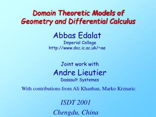
Domain Theory, Computational Geometry and Differential Calculus. Abbas Edalat Imperial College London www.doc.ic.ac.uk/~ae With contributions from Andre Lieutier, Ali Khanban, Marko Krznaric and Dirk Pattinson First SQU Workshop on Topology and its Applications December 2004.

Domain Theory, Computational Geometry and Differential Calculus
E N D
Presentation Transcript
Domain Theory, Computational Geometry and Differential Calculus Abbas Edalat Imperial College London www.doc.ic.ac.uk/~ae With contributions from Andre Lieutier, Ali Khanban, Marko Krznaric and Dirk Pattinson First SQU Workshop on Topology and its Applications December 2004
First rudimentary notion of a real number • In his ``Commentaries on the Difficulties in the Postulates of Euclid's Elements'', Omar Khayyam, the 11th century Persian mathematician and poet, first showed the equivalence of Euclid's notion of ratios with that of continued fractions. • Then, in a stroke of genius, he defined two ratios as equal ``when they can be expressed by the ratio of integer numbers with as great a degree of accuracy as we like.'' • Three centuries later, Ghiasseddin Jamshid Kashani, another Persian mathematician, devised the first fixed point technique for computation in analysis in the beginning of the 15th century: He used a cubic polynomial in a recursive scheme to approximate thesine of 1° correctly up to 17 decimal places
x {x} X Classical Space DXDomain Computational Model for Classical Spaces • Research project since 1993: Reconstruct mathematical analysis in an order-theoretic setting • Embed classical spaces into the set of maximal elements of suitable partially ordered sets, called domains:
Computational Model for Classical Spaces • Applications: Fractal Geometry Measure & Integration Theory: Generalized Riemann Integration Topological Representation of Spaces Exact Real Arithmetic Computational Geometry and Solid Modelling Differential Calculus Quantum Computation
Continuous Scott Domains • A directed complete partial order (dcpo) is a poset (A, ⊑) , in which every directed set {ai |iI } A has a sup or lub supiI ai • The way-below relation in a dcpo is defined by:a ≪ b iff for all directed subsets {ai |iI }, the relation b ⊑ supiI ai implies that there exists i Isuch that a ⊑ ai • If a ≪ b then a gives a finitary approximation to b • B A is a basis if for each a A , {b B | b ≪ a } is directed with lub a • A dcpo is(-)continuous if it has a (countable) basis • A dcpo is bounded complete if every bounded subset has a lub • A continuous Scott Domain is an -continuous bounded complete dcpo
Continuous functions • The Scott topology of a dcpo has as closed subsets downward closed subsets that are closed under the lub of directed subsets, usually only T0. Proposition. If D is a dcpo then f:D D is Scott continuous iff (i) f is monotone, i.e. f(x) ⊑ f(y) if x ⊑ y, and (ii) f preserves sups of directed subsets, i.e. for any directed set AD, we have: supaA f(a) = f(supA) • Fact. The Scott topology on a continuous dcpo A with basis B has basic open sets {a A | b ≪ a } for each b B.
{x} x x {x} : R IR an embedding We identify {x} with x R I R The Domain of nonempty compact Intervals of R Let IR={ [a,b] | a, b R} {R} (IR, ) is a bounded complete dcpo with R as bottom: supiI ai = iI ai a ≪ b ao b (IR, ⊑) is -continuous:countable basis {[p,q] | p < q & p, q Q} (IR, ⊑) is, thus, a continuous Scott domain. Scott topology has basis:↟a = {b | ao b}
Continuous Functions Scott continuous f:[0,1]n IR is given by lower and upper semi-continuous functions f -, f +:[0,1]n R with f(x)=[f -(x),f +(x)] f : [0,1]n R, f C0[0,1]n, has continuous extension i(f ): [0,1]n IR x {f (x)} Scott continuous maps [0,1]n IR with:f ⊑ g x R . f(x) ⊑ g(x)is another continuous Scott domain. The function space [0,1]n IR is a continuous Scott domain. : C0[0,1]n↪ ( [0,1]n IR), with f i(f) is a topological embedding into a proper subset of maximal elements of [0,1]n IR . We identify x and {x}, also f and i(f)
Single-stepfunction: a↘b : [0,1]n IR, with a I[0,1]n, b=[b-,b+] IR: b x ao x otherwise Step Functions Lubs of finite and bounded collections of single- step functions f= sup1in(ai ↘bi)are called step functions with N(f):= n (number of pieces) Step functions with ai, birational intervals give a basis for[0,1]n IR. They are used to approximate C0 functions.
Step Functions-An Example in R R b3 a3 b1 b2 a1 a2 0 1
Refining the Step Functions R b3 a3 b1 a1 b2 a2 0 1
Kleene’s Fixed Point Theorem • Theorem. If D is a dcpo with bottom (least element) d0 and if f : D D is Scott continuous then f has a least fixed point given by supiN f i(d0)
Initial Value Problems in Domain • Consider initial value problems given by where y=(y1,…,yn): [-a,a]Rn and v: [-K,K]n[-M,M]n are continuous.. • ODE solving: • Mathematical Analysis: no direct computational content • Numerical Analysis: no correctness guarantee • Interval Analysis: no convergence guarantee • Computable Analysis: no data types • Domain Theory provides a method which • is based on proper data types • has guaranteed speed of convergence • is directly implementable on a digital computer
Picard's Classical Theorem • Standard assumption: v: [-K, K]n [-M, M]n and aM ≤K. • Theorem: Suppose v is Lipschitz: |v(x) - v(y)| ≤ L |x – y| for some L > 0 and all x, y [-K, K]n. then, there exists a unique y: [-a, a] [-K, K]n with • Proof: For y: [-a, a] [-K, K]n let Pv(y): [-a, a] [-K, K]n with By Banach's fixed point theorem, the sequence yk defined by y0 = any initial continuous function, and yk+1 = Pv(yk) converges to the unique fixed point.
Translation to Domain Theory: Road map • Formulate the problem as fixed point equation over [-a,a]I[-K,K]n • Apply Kleene's Theorem to obtain the least fixed point • Relate domain-theoretic fixed points to the classical problem • Show that the computations restrict to bases of the involved domains. • Furthermore, we give: (i) Estimates on the speed of convergence (ii) Estimates on the (algebraic) complexity of the problem.
Translation to Domain Theory: Solutions • Interval valued approximations to the solution: • S = { y: [-a, a] I[-K, K]n | y Scott continuous} where • I[-K, K]n = {A | A [-K, K]n is a compact rectangle} is the sub-domain of rectangles contained in [-K, K]n with reverse inclusion. • The order on S is pointwise: • If f, g S then f ⊑ g iff f(x) ⊑ g(x) for all x [-a, a].
Translation into Domain Theory: Vector Field • Computing v(y) requires vector fields with interval input: • V= { u: I[-K, K]n I[-M, M]n | u Scott continuous } with pointwise ordering • Relationship to Classical Vector Fields: Extensions • u V extends a classical v: [-K, K]n [-M, M]n if • u({x}) = { v(x) } for all x [-K, K]n. • The greatest or canonical extension of v is given by Iv: I[-K, K]n I[-M, M]n with ((Iv)(A))i =vi[A]
The Domain Theoretic Picard Operator • Let u V. • The domain-theoretic Picard operator Pu:SS is given by where for f = [f- -, f +]: [-a, a] I[-K, K] • The monotone convergence theorem shows that Pu is Scott continuous.
Relationship to the Classical Problem • Assume u is an extension of v: [-K, K]n [-M, M]n. • Suppose y is the least fixed point of Pu • Every solution f satisfies y ⊑ f • If y = [y-, y+] and y- = y+, then y- is the unique solution. • That is, we look for fixed points of width 0: • For (A1, …..,An) I[-K, K]n, we write Ai = [Ai-, Ai+] and define the width of A by • w(A)=max{Ai+-Ai- | 1≤i≤n} • w(f)=sup{w(f(x))| x[-a,a]}
The Lipschitz Case • Recall: The classical proof assumes that v is Lipschitz. • Suppose u is interval Lipschitz, that is • w(u(x)) ≤L w(x) for all x I[-K, K]n. • Then w(Pu(y)) ≤ a L w(y) for all y S. • Assuming aL < 1 (which can be actually removed), we obtain • Theorem: y0 = [-K, K]n and yk+1 = Pu(yk). Theny = sup kN yk satisfies Pu(y) = y and w(y) = 0. • In particular, y - = y+ is the unique solution.
Theorem: Suppose u = supk uk and y0 = [-K, K]n and Approximations of the Vector Field • Proposition: The map P: V→(S→S) with u→ Pu is Scott continuous. • This allows us to use approximations of the vector field to obtain the solution: . Then y = sup k N yk satisfies Pu(y) =y and w(y) = 0. Speed of Convergence: • If aL < c < 1 and d(u, uk) < 2Mck (c - aL), then w(yk) ≤ck w(y0), where
Restrinting to a Base • Let a,K,MQ. • Denote the class of rational step functions I[-K,K]n→I[-M,M]n by VQ. • We also have the class SL Qof rational piecewise linear step functions f:[-a,a]→I[-K,K]n We again put N(f) = number of pieces in f In the above example N(f)=3
Computing with SLQ and VQ • Pu restricts to the base: • Suppose u VQ and y SLQ then: • The map u(y) is piecewise constant, hence Pu(y) SLQ Pu(y) SLQ . • Pu(y) can be computed in time O(N(u)N(y)), i.e. • N(Pu(y)) O(N(u)N(y)).
Summary • Suppose u = supk uk with ukVQ , y0= [-K, K]n and then • yk SLQ for all k N • y = supk yk has width 0 and is the unique solution • w(yk) O(ck) if d(u, uk) O(ck). • Given an elementary function u, one can use continued fractions for to obtain uk with the above properties.. • These properties are preserved in an implementation using rational arithmetic.
PART II: A Domain-Theoretic Model for Differential Calculus • Overall Aim:Synthesize Computer Science with Differential Calculus • Plan of the talk: • Primitives of continuous interval-valued function in Rn • Derivative of a continuous function in Rn • Fundamental Theorem of Calculus for interval-valued functions in Rn • Domain of C1 functions in Rn • Inverse and implicit functions in domain theory
Operations in Interval Arithmetic • For a = [a-, a+] IR, b = [b-, b+] IR,and * { +, –, } we have: a * b = { x*y | x a, y b } For example: • a + b = [a- + b-, a+ + b+] • Recall that for real x, we identify {x} with x.
Classically, with Basic Construction n=1 • What is a primitive map of a single step function a↘b ? We expect a↘b ([0,1] IR) For what f C1[0,1], should we have If a↘b ? f should satisfy:
Interval Lipschitz contant Assume f C1[0,1], a I[0,1], b IR. Supposex ao . b- f ′ (x) b+. We think of [b-, b+] as an interval Lipschitz constant for f at a. • Note thatx ao . b- f ′(x) b+ iff x1, x2 ao & x1 > x2 , b- (x1 – x2) f(x1) – f(x2) b+(x1 – x2), i.e. b(x1 – x2) ⊑ {f(x1) – f(x2)} = {f(x1)} – {f(x2)}
Proposition. For f: [0,1] IR, we have f (a,b) iff f(x) Maximal (IR) forx ao(hence f continuous)andGraph(f) is within lines of slopeb- & b+at each point (x, f(x)), x ao. . b+ (x, f(x)) Graph(f) b- a Definition of Interval Lipschitz constant • f ([0,1] IR) has an interval Lipschitz constantb IR at a I[0,1] ifx1, x2 ao, b(x1 – x2) ⊑ f(x1) – f(x2). • The tie of a with b, is (a,b) := { f | x1,x2 ao. b(x1 – x2) ⊑ f(x1) – f(x2)}
For Classical Functions Let f C1[0,1]; the following are equivalent: • f (a,b) • x ao . b- f ′(x) b+ • x1,x2 [0,1], x1,x2 ao. b(x1 – x2) ⊑ f (x1) – f (x2) • a↘b ⊑ f ′ Thus, (a,b) is our candidate for a↘b .
Set of primitive maps • : ([0,1] IR) (P([0,1] IR), ) ( Pthe power set constructor) • a↘b :=(a,b) • ⊔i Iai ↘bi := iI(ai,bi) • is well-defined and Scott continuous. • f is always a non-emptyset.
Definition. Given f : [0,1] IR the derivative of f is: : [0,1] IR = ⊔{a↘b | f (a,b) } • Theorem. (Compare with the classical case.) • is well–defined & Scott continuous. • If f C1[0,1], then • f (a,b) iff a↘b ⊑ The Derivative
Fundamental Theorem of Calculus • fg iff g(interval version) • If gC0 then fg iff g = (classical version) ⊑
Idea of Domain for C1Functions • If h C1[0,1] , then( h , h′ ) ([0,1] IR) ([0,1] IR) • We can approximate ( h, h′ ) in ([0,1] IR)2 i.e. ( f, g) ⊑ ( h ,h′ ) with f ⊑ h and g ⊑h′ • What pairs ( f, g) ([0,1] IR)2approximate a differentiable function?
Function and Derivative Consistency • Define the consistency relation:Cons ([0,1] IR) ([0,1] IR) with(f,g) Cons if (f) ( g) • Proposition (f,g) Cons iff there is a continuous h: dom(g) R with f ⊑ h and g ⊑ . In fact, if(f,g) Cons, there are least and greatest functions h with the above properties in each connected component of dom(g) which intersects dom(f) .
Define the upper envelop: s(f,g)(x) := supyOdom(f) S(f,g)(x,y) • Proposition. s(f,g) is the least function with f - s(f,g) and g ⊑ Consistency Test for (f,g) • For x dom(g), let g(x) = [g- (x), g+(x)] where g - , g+:dom(g) R are lower and upper semi-continuous. Similarly we define f -, f +:dom(f) R. Writef = [f –, f +]. Let O be a connected component of dom(g) with O dom(f) . For x , y O, let:
Similarly, let: • The lower envelop: t(f,g)(x) := inf yOdom(f) (f +(y) + T (f,g) (x,y)) • Proposition. t(f,g) is the greatest function with t(f,g) f+ and g⊑ • Theorem. (f, g) Con iff for all component O of dom(g) with O dom(f) and all x O. s (f, g) (x) t (f, g) (x).
t(f,g)= greatest function Approximating function: f = ⊔iai↘bi s(f,g) = least function Approximating derivative: g = ⊔j cj↘dj Consistency for basis elements (⊔iai↘bi, ⊔j cj↘dj) Cons is a finitary property:
f 1 1 g 2 1 Function and Derivative Information
f 1 1 g 2 1 Least and greatest functions
Proposition. For x O, we have:s(f,g)(x) = max {f –(x) , limsup f –(y) + S(f,g) (x , y) | ym O dom(f) } Decidability of consistency • For (f, g) = (⊔1inai↘bi , ⊔1jmcj↘dj), the rational end–points of aiand cj induce a partition y0 < y1 < y2 < … < ykof the connected component O of dom(g). • Hence s(f,g) is the max of k+2 rationallinear maps. • Similarly for t(f,g)(x). • Thus, s(f,g) t(f,g) is decidable. • Theorem. Consistency is decidable.
The Domain of C1Functions • Lemma.Cons ([0,1] IR)2is Scott closed. • Theorem.D1 [0,1]:= { (f,g) ([0,1]IR)2 | (f,g) Cons} is a continuous Scott domain, which can be given an effective structure. • Theorem. : C0[0,1] D1 [0,1] f (f , ) is topological embedding, giving a computational model for continuous functions and their differential properties. It restricts to give an embedding of C1[0,1].
Functions of several varibales • (IR)1× nrow n-vectors with entries in IR • For dcpo A, let(An)s = smash product of n copies of A:x(An)sif x=(x1,…..xn) with xi non-bottomor x=bottom • We work with (IR1× n)s
Definition of Interval Lipschitz constant • f ([0,1]n IR) has an interval Lipschitz constantb (IR1xn)sin a I[0,1]nifx, y ao, b(x – y) ⊑ f(x) – f(y). • The tie of a with b, is (a,b) := { f | x,y ao. b(x – y) ⊑ f(x) – f(y)} • Proposition. Iff(a,b), then f(x) Maximal (IR) forx aoand for all x,y ao. |f(x)-f(y)| k ||x-y|| with k=max i (|bi+|, |bi-|)
For Classical Functions Let f C1[0,1]n; the following are equivalent: • f (a,b) • x ao . b- f ´(x) b+ • x,y ao. b(x – y) ⊑ f (x) – f (y) • a↘b ⊑ f ′ Thus, (a,b) is our candidate for a↘b .
Set of primitive maps • : ([0,1]n IR) (P([0,1]n (IR1xn)s), ) ( Pthe power set constructor) • a↘b :=(a,b) • supi Iai ↘bi := iI(ai,bi) • is well-defined and Scott continuous. • g can be the empty set for 2 n Eg. g=(g1,g2), with g1(x , y)= y , g2(x, ,y)=0
Definition. Given f : [0,1]n IR the derivative of f is: : [0,1]n (IR1xn)s =sup{a↘b | f (a,b) } • Theorem. (Compare with the classical case.) • is well–defined & Scott continuous. • If f C1[0,1], then • f (a,b) iff a↘b ⊑ The Derivative
Fundamental Theorem of Calculus • fg iff g⊑(interval version) • If gC0 then fgiff g = (classical version)
Relation with Clarke’s gradient • For a locally Lipschitz f : [0,1]n IR • ∂ f (x)=convex{ lim mf ´(xm) | x mx} • It is a non-empty compact convex subset of Rn • Theorem: • For locally Lipschitzf : [0,1]n IR, the following holds: • The domain-theoretic derivativeat x , i.e. is the smallest n-dimensional rectangle with sides parallel to the coordinate planes that contains∂ f (x) • In dimension one the two coincide.