Domain Theory and Multi-Variable Calculus
This research project focuses on reconstructing mathematical analysis and integrating classical spaces into suitable domains. It incorporates concepts like Fractal Geometry, Topological Representation, and Quantum Computation. The talk covers topics from continuous functions to Scott Domains and Scott Topology. It explores various aspects of both differential calculus and computational modeling in classical spaces.

Domain Theory and Multi-Variable Calculus
E N D
Presentation Transcript
Domain Theory and Multi-Variable Calculus Abbas Edalat Imperial College London www.doc.ic.ac.uk/~ae Joint work with Andre Lieutier, Dirk Pattinson
x {x} X Classical Space DXDomain Computational Model for Classical Spaces • A research project since 1993: Reconstruct basic mathematical analysis • Embed classical spaces into the set of maximal elements of suitable domains
Computational Model for Classical Spaces • Other Applications: Fractal Geometry Measure & Integration Theory Topological Representation of Spaces Exact Real Arithmetic Computational Geometry and Solid Modelling Quantum Computation
A Domain-Theoretic Model for Differential Calculus • Overall Aim:Synthesize Computer Science with Differential Calculus • Plan of the talk: • Primitives of continuous interval-valued function in Rn • Derivative of a continuous function in Rn • Fundamental Theorem of Calculus for interval-valued functions in Rn • Domain of C1 functions in Rn • Inverse and implicit functions in domain theory
Continuous Scott Domains • A directed complete partial order (dcpo) is a poset (A, ⊑) , in which every directed set {ai |iI } A has a sup or lub ⊔iI ai • The way-below relation in a dcpo is defined by:a ≪ b iff for all directed subsets {ai |iI }, the relation b ⊑ ⊔iI ai implies that there exists i Isuch that a ⊑ ai • If a ≪ b then a gives a finitary approximation to b • B A is a basis if for each a A , {b B | b ≪ a } is directed with lub a • A dcpo is(-)continuous if it has a (countable) basis • A dcpo is bounded complete if every bounded subset has a lub • A continuous Scott Domain is an -continuous bounded complete dcpo
Continuous functions • The Scott topology of a dcpo has as closed subsets downward closed subsets that are closed under the lub of directed subsets, usually only T0. • Fact. The Scott topology on a continuous dcpo A with basis B has basic open sets {a A | b ≪ a } for each b B.
{x} x x {x} : R IRTopological embedding R I R The Domain of nonempty compact Intervals of R Let IR={ [a,b] | a, b R} {R} (IR, ) is a bounded complete dcpo with R as bottom: ⊔iI ai = iI ai a ≪ b ao b (IR, ⊑) is -continuous:countable basis {[p,q] | p < q & p, q Q} (IR, ⊑) is, thus, a continuous Scott domain. Scott topology has basis:↟a = {b | ao b}
Continuous Functions Scott continuous f:[0,1]n IR is given by lower and upper semi-continuous functions f -, f +:[0,1]n R with f(x)=[f -(x),f +(x)] f : [0,1]n R, f C0[0,1]n, has continuous extensionIf : [0,1]n IR x {f (x)} Scott continuous maps [0,1]n IR with:f ⊑ g x R . f(x) ⊑ g(x)is another continuous Scott domain. : C0[0,1]n↪ ( [0,1]n IR), with f Ifis a topological embedding into a proper subset of maximal elements of [0,1]n IR . We identify x and {x}, also f and If
Single-stepfunction: a↘b : [0,1]n IR, with a I[0,1]n, b=[b-,b+] IR: b x ao x otherwise Step Functions Lubs of finite and bounded collections of single- step functions ⊔1in(ai ↘bi)are called step functions. Step functions with ai, birational intervals, give a basis for[0,1]n IR. They are used to approximate C0 functions.
Step Functions-An Example in R R b3 a3 b1 b2 a1 a2 0 1
Refining the Step Functions R b3 a3 b1 a1 b2 a2 0 1
Graph(f) is within lines of slope b- & b+at each point (x, f(x)), x ao. . b+ (x, f(x)) b- Graph(f) a Interval Lipschitz constant in dimension one For f ([0,1] IR) we have: x1, x2 ao, b(x1 – x2) ⊑ f(x1) – f(x2) iff for all x2x1 b- (x1 – x2) f(x1) – f(x2) b+(x1 – x2) iff
Functions of several varibales • (IR)1× nrow n-vectors with entries in IR • For dcpo A, let (An)s = smash product of n copies of A:x(An)sif x=(x1,…..xn) with xi non-bottom for all i or x=bottom • Interval Lipschitz constants of real-valued functions in Rn take values in (IR1× n)s
Interval Lipschitz constant in R n • f ([0,1]n IR) has an interval Lipschitz constantb (IR1xn)sin a I[0,1]nifx, y ao, b(x – y) ⊑ f(x) – f(y). • The tie of a with b, is (a,b) := { f | x,y ao. b(x – y) ⊑ f(x) – f(y)} • Proposition. Iff(a,b), then f(x) Maximal (IR) forx aoand for all x,y ao. |f(x)-f(y)| k ||x-y|| with k=max i (|bi+|, |bi-|)
For Classical Functions Let f C1[0,1]n; the following are equivalent: • f (a,b) • x ao . b- f ´(x) b+ • x,y ao , b(x – y) ⊑ f (x) – f (y) • a↘b ⊑ f´ Thus, (a,b) is our candidate for a↘b .
Set of primitive maps • : ([0,1]n IR) (P([0,1]n (IR1xn)s), ) ( Pthe power set constructor) • a↘b :=(a,b) • ⊔i Iai ↘bi := iI(ai,bi) • is well-defined and Scott continuous. • g can be the empty set for 2 n Eg. g=(g1,g2), with g1(x , y)= y , g2(x ,y)=0
Definition. Given f : [0,1]n IR the derivative of f is: : [0,1]n (IR1xn)s = ⊔{a↘b | f (a,b) } • Theorem. (Compare with the classical case.) • is well–defined & Scott continuous. • If f C1[0,1], then • f (a,b) iff a↘b ⊑ The Derivative
Relation with Clarke’s gradient • For a locally Lipschitz f : [0,1]n R • ∂ f (x) := convex-hull{ lim mf ´(xm) | x mx} • It is a non-empty compact convex subset of Rn • Theorem: • For locally Lipschitzf : [0,1]n R • The domain-theoretic derivativeat x is the smallest n-dimensional rectangle with sides parallel to the coordinate planes that contains∂ f (x) • In dimension one, the two notions coincide.
x2=x1/2 (-1,1) r=([-1,0],[-1,1]) ([-1,1],[-1,1]) (0, -1) t=([-1,1],[0,1]) s=([0,1],[-1,0]) (1,0) x2=x1 x2=2x1 In dimension two • f: R2Rwithf(x1, x2) = max ( min (x1, x2) , x2-x1) ∂ f (0)= convex((-1,1),(-1,0),(01))
fg iff g⊑(interval version) • If gC0 then fgiff g = (classical version) Fundamental Theorem of Calculus
Idea of Domain for C1Functions • If h C1[0,1]n , then( h , h´ ) ([0,1]n IR) ([0,1]n IR)ns • We can approximate ( h, h´ ) in ([0,1]n IR) ([0,1]n IR)ns i.e. ( f, g) ⊑ ( h ,h´ ) with f ⊑ h and g ⊑h´ • What pairs ( f, g) ([0,1]n IR) ([0,1]n IR)ns approximate a differentiable function?
Proposition (f,g) Cons iff there is a continuous h: dom(g) R with f ⊑ h and g ⊑ . Function and Derivative Consistency • Define the consistency relation:Cons ([0,1]n IR) ([0,1]n IR)nswith(f,g) Cons if (f) ( g) In fact, if(f,g) Cons, there are least and greatest functions h with the above properties in each connected component of dom(g) which intersects dom(f) .
t(f,g)= greatest function Approximating function: f = ⊔iai↘bi s(f,g) = least function Approximating derivative: g = ⊔j cj↘dj Consistency in dimension one (⊔iai↘bi, ⊔j cj↘dj) Cons is a finitary property:
f 1 1 g 2 1 Function and Derivative Information
f 1 1 g 2 1 Least and greatest functions
f We solve: = v(t,x), x(t0) =x0 for t[0,1] with v(t,x) = tandt0=1/2, x0=9/8. 1 b2 b1 b3 a3 a2 a1 1 g v1 1 v2 v3 1 Solving Initial Value Problems v is approximated by a sequence of step functions, v0, v1, … v = ⊔ivi . t The initial condition is approximated by rectangles aibi: {(1/2,9/8)} =⊔i aibi, v t
f 1 1 g 1 1 Solution .
f 1 1 g 1 1 Solution .
f 1 1 g 1 1 Solution .
[-2,2] [-1,1] [-3,3] [-2,2] Basis of ([0,1]n IR) ([0,1]n IR)ns • Definition. g:[0,1]n (IRn)s the domain of g is dom(g) = {x | g(x) non-bottom} • Basis element: (f, g1,g2,….,gn) ([0,1]n IR) ([0,1]n IR)ns • Each f, gi :[0,1]n IR is a rational step function. • dom(g) is partitioned by disjoint crescents (intersection of closed and open sets) in each of which g is a constant rational interval. Eg. For n=2:A step function gi with four single stepfunctions with two horizontal and twovertical rectangles as their domainsand a hole inside, and with eight vertices.
Decidability of Consistency • (f,g) Cons if (f) ( g) • First we check if g is integrable, i.e. if g • In classical calculus, g:[0,1]n Rnwill be integrable by Green’s theorem iff for any piecewise smooth closed non-intersecting path • p:[0,1] [0,1]nwith p(0)=p(1) • We generalize this to type g:[0,1]n (IRn)s
Interval-valued path integral • For vIRn , uRn define the interval-valued scalar product
Generalized Green’s Theorem • Definition. g:[0,1]n (IRn)s the domain of g is dom(g) = {x | g(x) non-bottom} • Theorem. g iff for any piecewise smooth non-intersecting path p:[0,1] dom(g) with p(0)=p(1), we have zero-containment: • We can replace piecewise smooth with piecewise linear. • For step functions, the lower and upper path integrals will depend linearly on the nodes of the path, so their extreme values will be reached when these nodes are at the corners of dom(g). • Since there are finitely many of these extreme paths, zero containment can be decided in finite time for all paths.
.x y. Locally minimal paths • Definition. Given x,ydom(g), a non-self-intersecting pathp:[0,1] closure(dom(g)) with p(0)=y and p(1)=x islocally minimal if its length is minimal in its homotopicclass of paths from y to x.
Theorem. If g satisfies the zero-containment condition, then there is a non-self-intersecting locally minimal piecewise linear path p with • Vg (y ,y)=0 and g ⊑ Minimal surface • Step function g:[0,1]n (IRn)s . Let O be a component of dom(g) . Let x,yclosure(O). • Consider the following supremum over all piecewise linear paths p in closure(O) with p(0 )= y and p(1)= x. • For fixed y, the map Vg (. ,y): cl(O) R is a rational piecewise linear function. • It is the least continuous function or surface with:
Theorem. If g satisfies the zero-containment condition, then there is a non-self- intersecting locally minimal piecewise linear path q with • For fixed y, the map Wg (. ,y): cl(O) R is a rational piecewise linear function. • It is the greatest continuous function or surface with: • Wg (y ,y)=0 and g ⊑ Maximal surface • Step function g:[0,1]n (IRn)s . Let O be a component of dom(g) . Let x,ycl(O). • Consider the following infimum over all piecewise linear paths p in cl(O) with p(0 )= y and p(1)= x.
Put • Proposition. • Theorem. s(f,g): dom(g)R is the least continuous function with f - s(f,g) and g ⊑ Minimal surface for (f,g) • (f,g)([0,1]n IR) ([0,1]n IR)nsrational step function • Assume we have determined that g
Theorem. t(f,g): dom(g)R is the least continuous function with t(f,g) f +and g ⊑ Maximal surface for (f,g)
Decidability of Consistency • Theorem. Consistency is decidable. Proof: In s(f,g)t(f,g) we compare two rational piecewise-linear surfaces, which is decidable.
Theorem. : C0[0,1]n D1 [0,1]n f (f , ) is topological embedding into maximal elements of D1 , giving a computational model for continuous functions and their differential properties. The Domain of C1Functions • Lemma.Cons ([0,1]n IR) ([0,1]n IR)nsis Scott closed. • Theorem.D1 [0,1]n:= { (f,g) | (f,g) Cons} is a continuous Scott domain that can be given an effective structure.
Theorem. Let f:[-1,1]nRn such that the mean derivative M of f at 0 is invertible with || M-1 -I ||<1/n. Then: • The map f has a Lipschitz inverse in a neighbourhood of 0 . • Given an increasing sequence of step functions converging to f we can effectively obtain an increasing sequence of step functions converging to f-1 • If f is C1 and given also an increasing sequence of step functions converging to f ´we can also effectively obtain an increasing sequence of step functions converging to (f-1)' Inverse and Implicit Function theorems • Definition. Givenf:[-1,1]nRn the mean derivative at x0 is the linear map represented by the matrix M with Mij=
Further Work • A robust CAD • PDE’s • Differential Topology • Differential Geometry
THE END http://www.doc.ic.ac.uk/~ae