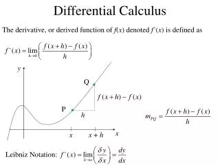
Differential calculus
Differential calculus. Differential calculus is concerned with the rate at which things change. For example, the speed of a car is the rate at which the distance it travels changes with time. First we shall review the gradient of a straight line graph, which represents a rate of change.

Differential calculus
E N D
Presentation Transcript
Differential calculus is concerned with the rate at which things change. For example, the speed of a car is the rate at which the distance it travels changes with time. First we shall review the gradient of a straight line graph, which represents a rate of change.
Gradient of a straight line graph The gradient of the line between two points (x1, y1) and (x2, y2) is where m is a fixed number called a constant. A gradient can be thought of as the rate of change of y with respect to x.
Gradient of a curve A curve does not have a constant gradient. Its direction is continuously changing, so its gradient will continuously change too. y = f(x) The gradient of a curve at any point on the curve is defined as being the gradient of the tangent to the curve at this point.
Tangent to the curve at A. y A O x A tangent is a straight line, which touches, but does not cut, the curve. We cannot calculate the gradient of a tangent directly , as we know only one point on the tangent and we require two points to calculate the gradient of a line.
y Tangent to the curve at A. A O x Using geometry to approximate to a gradient Look at this curve. B1 B2 B3 Look at the chords AB1, AB2, AB3, . . . For points B1, B2, B3, . . . that are closer and closer to A the sequence of chords AB1, AB2, AB3, . . . move closer to becoming the tangent at A. The gradients of the chords AB1, AB2, AB3, . . . move closer to becoming the gradient of the tangent at A.
B4 (2.001, 4.004001) B2 (2.5, 6.25) B3 (2.1, 4.41) A numerical approach to rates of change Here is how the idea can be applied to a real example. Look at the section of the graph of y = x2 for 2 >x> 3. We want to find the gradient of the curve at A(2, 4). B1(3, 9) 4 to 9 = 5 2 to 3 4 to 6.25 = 4.5 2 to 2.5 = 4.1 2 to 2.1 4 to 4.41 Complete the table A (2, 4) The gradient of the chord AB1 is 4 to 4.004001 = 4.001 2 to 2.001 2 to 2.00001 4 to 4.0000400001 4.00001
y y = x2 4 2 x As the points B1, B2, B3, . . . get closer and closer to A the gradient is getting closer to 4. This suggests that the gradient of the curve y = x2 at the point (2, 4) is 4.
I’d guess 2. (1, ) Example (1) Find the gradient of the chord joining the two points with x-coordinates 1 and 1.001 on the graph of y = x2. Make a guess about the gradient of the tangent at the point x = 1. The gradient of the chord is (1.001, ) 1.0012 = 2.001 1)
I’d guess 16. (8, ) Example (2) Find the gradient of the chord joining the two points with x-coordinates 8 and 8.0001 on the graph of y = x2. Make a guess about the gradient of the tangent at the point x = 8. The gradient of the chord is (8.0001, ) 8.00012 = 16.0001 64
Let’s make a table of the results so far: You’re probably noticing a pattern here. But can we prove it mathematically?
I will call it ∆x. (2, 4) h I need to consider what happens when I increase x by a general increment. I will call it h. (2 + h, (2 + h)2)
y y = x2 B(2 + h, (2 + h)2) A(2, 4) O x If h≠ 0 we can cancel the h’s. Let y = x2 and let A be the point (2, 4) Let B be the point (2 + h, (2 + h)2) Here we have increased x by a very small amount h. In the early days of calculus h was referred to as an infinitesimal. Draw the chord AB. Gradient of AB Use a similar method to find the gradient of y = x2 at the points (i) (3, 9) (ii) (4, 16) = 4 + h As h approaches zero, 4 + h approaches 4. So the gradient of the curve at the point (2, 4) is 4.
It looks like the gradient is simply 2x. We can now add to our table: 6 8
Let’s check this result. y = x2
Let’s check this result. y = x2 Gradient at (3, 9) = 6
Let’s check this result. y = x2 Gradient at (2, 4) = 4
Let’s check this result. y = x2 Gradient at (1, 1) = 2
Let’s check this result. y = x2 Gradient at (0, 0) = 0
Let’s check this result. y = x2 Gradient at (–1, 1) = –2
Let’s check this result. y = x2 Gradient at (–2, 4) = –4
Let’s check this result. y = x2 Gradient at (–3, 9) = –6
ZOOM IN Another way of seeing what the gradient is at the point (2, 4) is to plot an accurate graph and ‘zoom in’. y = x2
When we zoom in the curve starts to look like a straight line which makes it easy to estimate the gradient. 0.8 0.2