Download
1 / 72
720 likes | 891 Vues
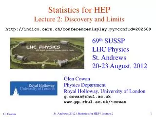
Statistics for HEP Lecture 2: Discovery and Limits. http://indico.cern.ch/conferenceDisplay.py?confId=202569. 69 th SUSSP LHC Physics St. Andrews 20-23 August, 2012. Glen Cowan Physics Department Royal Holloway, University of London g.cowan@rhul.ac.uk www.pp.rhul.ac.uk/~cowan.

E N D
Statistics for HEPLecture 2: Discovery and Limits http://indico.cern.ch/conferenceDisplay.py?confId=202569 69th SUSSP LHC Physics St. Andrews 20-23 August, 2012 Glen Cowan Physics Department Royal Holloway, University of London g.cowan@rhul.ac.uk www.pp.rhul.ac.uk/~cowan St. Andrews 2012 / Statistics for HEP / Lecture 2 TexPoint fonts used in EMF. Read the TexPoint manual before you delete this box.: AAAA
Outline Lecture 1: Introduction and basic formalism Probability, statistical tests, parameter estimation. Lecture 2: Discovery and Limits Quantifying discovery significance and sensitivity Frequentist and Bayesian intervals/limits Lecture 3: Further topics The Look-Elsewhere Effect Unfolding (deconvolution) St. Andrews 2012 / Statistics for HEP / Lecture 2
Recap on statistical tests Consider test of a parameter μ, e.g., proportional to signal rate. Result of measurement is a set of numbers x. To define testofμ, specify critical regionwμ, such that probability to find x∈ wμ is not greater than α (the size or significance level): (Must use inequality since x may be discrete, so there may not exist a subset of the data space with probability of exactly α.) Equivalently define a p-value pμ such that the critical region corresponds to pμ ≤ α. Often use, e.g., α = 0.05. If observe x∈ wμ, reject μ. St. Andrews 2012 / Statistics for HEP / Lecture 1
Cowan, Cranmer, Gross, Vitells, arXiv:1007.1727, EPJC 71 (2011) 1554 Large-sample approximations for prototype analysis using profile likelihood ratio Search for signal in a region of phase space; result is histogram of some variable x giving numbers: Assume the ni are Poisson distributed with expectation values strength parameter where signal background St. Andrews 2012 / Statistics for HEP / Lecture 2
Prototype analysis (II) Often also have a subsidiary measurement that constrains some of the background and/or shape parameters: Assume the mi are Poisson distributed with expectation values nuisance parameters (θs, θb,btot) Likelihood function is St. Andrews 2012 / Statistics for HEP / Lecture 2
The profile likelihood ratio Base significance test on the profile likelihood ratio: maximizes L for Specified μ maximize L The likelihood ratio of point hypotheses gives optimum test (Neyman-Pearson lemma). The profile LR in the present analysis with variable μ and nuisance parameters θ is expected to be near optimal. St. Andrews 2012 / Statistics for HEP / Lecture 2
Test statistic for discovery Try to reject background-only (μ= 0) hypothesis using i.e. here only regard upward fluctuation of data as evidence against the background-only hypothesis. Note that even though here physically m ≥ 0, we allow to be negative. In large sample limit its distribution becomes Gaussian, and this will allow us to write down simple expressions for distributions of our test statistics. St. Andrews 2012 / Statistics for HEP / Lecture 2
p-value for discovery Large q0 means increasing incompatibility between the data and hypothesis, therefore p-value for an observed q0,obs is will get formula for this later From p-value get equivalent significance, St. Andrews 2012 / Statistics for HEP / Lecture 2
Expected (or median) significance / sensitivity When planning the experiment, we want to quantify how sensitive we are to a potential discovery, e.g., by given median significance assuming some nonzero strength parameter μ′. So for p-value, need f(q0|0), for sensitivity, will need f(q0|μ′), St. Andrews 2012 / Statistics for HEP / Lecture 2
Cowan, Cranmer, Gross, Vitells, arXiv:1007.1727, EPJC 71 (2011) 1554 Distribution of q0 in large-sample limit Assuming approximations valid in the large sample (asymptotic) limit, we can write down the full distribution of q0 as The special case μ′ = 0 is a “half chi-square” distribution: In large sample limit, f(q0|0) independent of nuisance parameters; f(q0|μ′) depends on nuisance parameters through σ. St. Andrews 2012 / Statistics for HEP / Lecture 2
Cowan, Cranmer, Gross, Vitells, arXiv:1007.1727, EPJC 71 (2011) 1554 Cumulative distribution of q0, significance From the pdf, the cumulative distribution of q0 is found to be The special case μ′ = 0 is The p-value of the μ = 0 hypothesis is Therefore the discovery significance Z is simply St. Andrews 2012 / Statistics for HEP / Lecture 2
Test statistic for upper limits For purposes of setting an upper limit on μ one may use where Note for purposes of setting an upper limit, one does not regard an upwards fluctuation of the data as representing incompatibility with the hypothesized μ. From observed qm find p-value: 95% CL upper limit on m is highest value for which p-value is not less than 0.05. St. Andrews 2012 / Statistics for HEP / Lecture 2
Cowan, Cranmer, Gross, Vitells, arXiv:1007.1727, EPJC 71 (2011) 1554 Distribution ofqμ in large-sample limit Independent of nuisance parameters. St. Andrews 2012 / Statistics for HEP / Lecture 2
Cowan, Cranmer, Gross, Vitells, arXiv:1007.1727, EPJC 71 (2011) 1554 Monte Carlo test of asymptotic formula Here take τ = 1. Asymptotic formula is good approximation to 5σ level (q0 = 25) already for b ~ 20. St. Andrews 2012 / Statistics for HEP / Lecture 2
Cowan, Cranmer, Gross, Vitells, arXiv:1007.1727, EPJC 71 (2011) 1554 Monte Carlo test of asymptotic formulae Consider again n ~ Poisson (μs + b), m ~ Poisson(τb) Use qμ to find p-value of hypothesized μ values. E.g. f (q1|1) for p-value of μ=1. Typically interested in 95% CL, i.e., p-value threshold = 0.05, i.e., q1 = 2.69 or Z1 = √q1 = 1.64. Median[q1 |0] gives “exclusion sensitivity”. Here asymptotic formulae good for s = 6, b = 9. St. Andrews 2012 / Statistics for HEP / Lecture 2
Unified (Feldman-Cousins) intervals We can use directly where as a test statistic for a hypothesized μ. Large discrepancy between data and hypothesis can correspond either to the estimate for μ being observed high or low relative to μ. This is essentially the statistic used for Feldman-Cousins intervals (here also treats nuisance parameters). G. Feldman and R.D. Cousins, Phys. Rev. D 57 (1998) 3873. St. Andrews 2012 / Statistics for HEP / Lecture 2
Distribution of tμ Using Wald approximation, f (tμ|μ′) is noncentral chi-square for one degree of freedom: Special case of μ = μ′ is chi-square for one d.o.f. (Wilks). The p-value for an observed value of tμ is and the corresponding significance is St. Andrews 2012 / Statistics for HEP / Lecture 2
Low sensitivity to μ It can be that the effect of a given hypothesized μ is very small relative to the background-only (μ = 0) prediction. This means that the distributions f(qμ|μ) and f(qμ|0) will be almost the same: St. Andrews 2012 / Statistics for HEP / Lecture 2
Having sufficient sensitivity In contrast, having sensitivity to μ means that the distributions f(qμ|μ) and f(qμ|0) are more separated: That is, the power (probability to reject μ if μ = 0) is substantially higher than α. Use this power as a measure of the sensitivity. St. Andrews 2012 / Statistics for HEP / Lecture 2
Spurious exclusion Consider again the case of low sensitivity. By construction the probability to reject μ if μ is true is α (e.g., 5%). And the probability to reject μ if μ= 0 (the power) is only slightly greater than α. This means that with probability of around α = 5% (slightly higher), one excludes hypotheses to which one has essentially no sensitivity (e.g., mH = 1000 TeV). “Spurious exclusion” St. Andrews 2012 / Statistics for HEP / Lecture 2
Ways of addressing spurious exclusion The problem of excluding parameter values to which one has no sensitivity known for a long time; see e.g., In the 1990s this was re-examined for the LEP Higgs search by Alex Read and others and led to the “CLs” procedure for upper limits. Unified intervals also effectively reduce spurious exclusion by the particular choice of critical region. St. Andrews 2012 / Statistics for HEP / Lecture 2
The CLs procedure In the usual formulation of CLs, one tests both the μ = 0 (b) and μ > 0 (μs+b) hypotheses with the same statistic Q = -2ln Ls+b/Lb: f (Q|b) f (Q| s+b) ps+b pb St. Andrews 2012 / Statistics for HEP / Lecture 2
The CLs procedure (2) As before, “low sensitivity” means the distributions of Q under b and s+b are very close: f (Q|b) f (Q|s+b) ps+b pb St. Andrews 2012 / Statistics for HEP / Lecture 2
The CLs procedure (3) The CLs solution (A. Read et al.) is to base the test not on the usual p-value (CLs+b), but rather to divide this by CLb (~ one minus the p-value of the b-only hypothesis), i.e., f (Q|s+b) Define: f (Q|b) 1-CLb = pb CLs+b = ps+b Reject s+b hypothesis if: Reduces “effective”p-value when the two distributions become close (prevents exclusion if sensitivity is low). St. Andrews 2012 / Statistics for HEP / Lecture 2
Setting upper limits on μ=σ/σSM Carry out the CL“s” procedure for the parameter μ = σ/σSM, resulting in an upper limit μup. In, e.g., a Higgs search, this is done for each value of mH. At a given value of mH, we have an observed value of μup, and we can also find the distribution f(μup|0): ±1σ (green) and ±2σ (yellow) bands from toy MC; Vertical lines from asymptotic formulae. St. Andrews 2012 / Statistics for HEP / Lecture 2
How to read the green and yellow limit plots For every value of mH, find the CLs upper limit on μ. Also for each mH, determine the distribution of upper limits μup one would obtain under the hypothesis of μ = 0. The dashed curve is the median μup, and the green (yellow) bands give the ± 1σ (2σ) regions of this distribution. ATLAS, Phys. Lett. B 710 (2012) 49-66 St. Andrews 2012 / Statistics for HEP / Lecture 2
How to read the p0 plot The “local”p0 means the p-value of the background-only hypothesis obtained from the test of μ = 0 at each individual mH, without any correct for the Look-Elsewhere Effect. The “Sig. Expected” (dashed) curve gives the median p0 under assumption of the SM Higgs (μ = 1) at each mH. ATLAS, Phys. Lett. B 710 (2012) 49-66 St. Andrews 2012 / Statistics for HEP / Lecture 2
How to read the “blue band” On the plot of versus mH, the blue band is defined by i.e., it approximates the 1-sigma error band (68.3% CL conf. int.) ATLAS, Phys. Lett. B 710 (2012) 49-66 St. Andrews 2012 / Statistics for HEP / Lecture 2
The Bayesian approach to limits In Bayesian statistics need to start with ‘prior pdf’p(q), this reflects degree of belief about q before doing the experiment. Bayes’ theorem tells how our beliefs should be updated in light of the data x: Integrate posterior pdf p(q | x) to give interval with any desired probability content. For e.g. n ~ Poisson(s+b), 95% CL upper limit on s from St. Andrews 2012 / Statistics for HEP / Lecture 2
Bayesian prior for Poisson parameter Include knowledge that s≥0 by setting prior p(s) = 0 for s<0. Could try to reflect ‘prior ignorance’ with e.g. Not normalized but this is OK as long as L(s) dies off for large s. Not invariant under change of parameter — if we had used instead a flat prior for, say, the mass of the Higgs boson, this would imply a non-flat prior for the expected number of Higgs events. Doesn’t really reflect a reasonable degree of belief, but often used as a point of reference; or viewed as a recipe for producing an interval whose frequentist properties can be studied (coverage will depend on true s). St. Andrews 2012 / Statistics for HEP / Lecture 2
Bayesian interval with flat prior for s Solve numerically to find limit sup. For special case b = 0, Bayesian upper limit with flat prior numerically same as one-sided frequentist case (‘coincidence’). Otherwise Bayesian limit is everywhere greater than the one-sided frequentist limit, and here (Poisson problem) it coincides with the CLs limit. Never goes negative. Doesn’t depend on b if n = 0. St. Andrews 2012 / Statistics for HEP / Lecture 2
Priors from formal rules Because of difficulties in encoding a vague degree of belief in a prior, one often attempts to derive the prior from formal rules, e.g., to satisfy certain invariance principles or to provide maximum information gain for a certain set of measurements. Often called “objective priors” Form basis of Objective Bayesian Statistics The priors do not reflect a degree of belief (but might represent possible extreme cases). In Objective Bayesian analysis, can use the intervals in a frequentist way, i.e., regard Bayes’ theorem as a recipe to produce an interval with certain coverage properties. St. Andrews 2012 / Statistics for HEP / Lecture 2
Priors from formal rules (cont.) For a review of priors obtained by formal rules see, e.g., Formal priors have not been widely used in HEP, but there is recent interest in this direction, especially the reference priors of Bernardo and Berger; see e.g. L. Demortier, S. Jain and H. Prosper, Reference priors for high energy physics, Phys. Rev. D 82 (2010) 034002, arXiv:1002.1111. D. Casadei, Reference analysis of the signal + background model in counting experiments, JINST 7 (2012) 01012; arXiv:1108.4270. St. Andrews 2012 / Statistics for HEP / Lecture 2
Jeffreys’ prior According to Jeffreys’rule, take prior according to where is the Fisher information matrix. One can show that this leads to inference that is invariant under a transformation of parameters. For a Gaussian mean, the Jeffreys’ prior is constant; for a Poisson mean m it is proportional to 1/√m. St. Andrews 2012 / Statistics for HEP / Lecture 2
Jeffreys’ prior for Poisson mean Suppose n ~ Poisson(m). To find the Jeffreys’ prior for m, So e.g. for m = s + b, this means the prior p(s) ~ 1/√(s + b), which depends on b. Note this is not designed as a degree of belief about s. St. Andrews 2012 / Statistics for HEP / Lecture 2
L (x|θ) Nuisance parameters In general our model of the data is not perfect: model: truth: x Can improve model by including additional adjustable parameters. Nuisance parameter ↔ systematic uncertainty. Some point in the parameter space of the enlarged model should be “true”. Presence of nuisance parameter decreases sensitivity of analysis to the parameter of interest (e.g., increases variance of estimate). St. Andrews 2012 / Statistics for HEP / Lecture 3
p-values in cases with nuisance parameters Suppose we have a statistic qθ that we use to test a hypothesized value of a parameter θ, such that the p-value of θ is But what values of ν to use for f(qθ|θ, ν)? Fundamentally we want to reject θ only if pθ < α for all ν. → “exact” confidence interval Recall that for statistics based on the profile likelihood ratio, the distribution f(qθ|θ, ν) becomes independent of the nuisance parameters in the large-sample limit. But in general for finite data samples this is not true; one may be unable to reject some θ values if all values of ν must be considered, even those strongly disfavoured by the data (resulting interval for θ“overcovers”). St. Andrews 2012 / Statistics for HEP / Lecture 3
Profile construction (“hybrid resampling”) Compromise procedure is to reject θ if pθ ≤ αwhere the p-value is computed assuming the value of the nuisance parameter that best fits the data for the specified θ: “double hat” notation means value of parameter that maximizes likelihood for the given θ. The resulting confidence interval will have the correct coverage for the points . Elsewhere it may under- or overcover, but this is usually as good as we can do (check with MC if crucial or small sample problem). St. Andrews 2012 / Statistics for HEP / Lecture 3
“Hybrid frequentist-Bayesian” method Alternatively, suppose uncertainty in ν is characterized by a Bayesian prior π(ν). Can use the marginal likelihood to model the data: This does not represent what the data distribution would be if we “really” repeated the experiment, since then ν would not change. But the procedure has the desired effect. The marginal likelihood effectively builds the uncertainty due to ν into the model. Use this now to compute (frequentist) p-values → result has hybrid “frequentist-Bayesian” character. St. Andrews 2012 / Statistics for HEP / Lecture 3
The “ur-prior” behind the hybrid method But where did π(ν) come frome? Presumably at some earlier point there was a measurement of some data y with likelihood L(y|ν), which was used in Bayes’theorem, and this “posterior” was subsequently used for π(ν) for the next part of the analysis. But it depends on an “ur-prior”π0(ν), which still has to be chosen somehow (perhaps “flat-ish”). But once this is combined to form the marginal likelihood, the origin of the knowledge of ν may be forgotten, and the model is regarded as only describing the data outcome x. St. Andrews 2012 / Statistics for HEP / Lecture 3
The (pure) frequentist equivalent In a purely frequentist analysis, one would regard both x and y as part of the data, and write down the full likelihood: “Repetition of the experiment” here means generating both x and y according to the distribution above. In many cases, the end result from the hybrid and pure frequentist methods are found to be very similar (cf. Conway, Roever, PHYSTAT 2011). St. Andrews 2012 / Statistics for HEP / Lecture 3
More on priors Suppose we measure n ~ Poisson(s+b), goal is to make inference about s. Suppose b is not known exactly but we have an estimate bmeas with uncertainty sb. For Bayesian analysis, first reflex may be to write down a Gaussian prior for b, But a Gaussian could be problematic because e.g. b ≥ 0, so need to truncate and renormalize; tails fall off very quickly, may not reflect true uncertainty. St. Andrews 2012 / Statistics for HEP / Lecture 3
Bayesian limits on s with uncertainty on b Consider n ~ Poisson(s+b) and take e.g. as prior probabilities Put this into Bayes’ theorem, Marginalize over the nuisance parameter b, Then use p(s|n) to find intervals for s with any desired probability content. St. Andrews 2012 / Statistics for HEP / Lecture 3
Gamma prior for b What is in fact our prior information about b? It may be that we estimated b using a separate measurement (e.g., background control sample) with m ~ Poisson(tb) (t = scale factor, here assume known) Having made the control measurement we can use Bayes’ theorem to get the probability for b given m, If we take the ur-prior p0(b) to be to be constant for b ≥ 0, then the posterior p(b|m), which becomes the subsequent prior when we measure n and infer s, is a Gamma distribution with: mean = (m + 1) /t standard dev. = √(m + 1) /t St. Andrews 2012 / Statistics for HEP / Lecture 3
Gamma distribution St. Andrews 2012 / Statistics for HEP / Lecture 3
Frequentist test with Bayesian treatment of b Distribution of n based on marginal likelihood (gamma prior for b): and use this as the basis of a test statistic: p-values from distributions of qm under background-only (0) or signal plus background (1) hypotheses: St. Andrews 2012 / Statistics for HEP / Lecture 3
Frequentist approach to same problem In the frequentist approach we would regard both variables n ~ Poisson(s+b) m ~ Poisson(tb) as constituting the data, and thus the full likelihood function is Use this to construct test of s with e.g. profile likelihood ratio Note here that the likelihood refers to both n and m, whereas the likelihood used in the Bayesian calculation only modeled n. St. Andrews 2012 / Statistics for HEP / Lecture 3
Test based on fully frequentist treatment Data consist of both n and m, with distribution Use this as the basis of a test statistic based on ratio of profile likelihoods: Here combination of two discrete variables (n and m) results in an approximately continuous distribution for qp. St. Andrews 2012 / Statistics for HEP / Lecture 3
Log-normal prior for systematics In some cases one may want a log-normal prior for a nuisance parameter (e.g., background rate b). This would emerge from the Central Limit Theorem, e.g., if the true parameter value is uncertain due to a large number of multiplicative changes, and it corresponds to having a Gaussian prior for β = ln b. whereβ0 = ln b0 and in the following we write σ as σβ. St. Andrews 2012 / Statistics for HEP / Lecture 3
The log-normal distribution St. Andrews 2012 / Statistics for HEP / Lecture 3