Bayesian inference
290 likes | 443 Vues
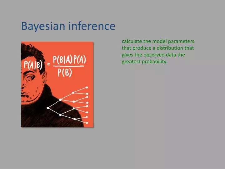
Bayesian inference. calculate the model parameters that produce a distribution that gives the observed data the greatest probability. Thomas Bayes. Bayesian methods were invented in the 18 th century , but their application in phylogenetics dates from 1996. Thomas Bayes ? (1701?-1761?).

Bayesian inference
E N D
Presentation Transcript
Bayesianinference calculate the model parameters that produce a distribution that gives the observed data the greatest probability
Thomas Bayes Bayesian methods were invented in the 18thcentury, but their application in phylogenetics dates from 1996. Thomas Bayes? (1701?-1761?)
Bayes’ theorem Bayes’ theorema links a conditional probability to its inverse Prob(H) Prob(D|H) Prob(H|D) = ∑HProb(H) Prob(D|H)
Bayes’ theorem in the case of two alternative hypotheses, the theorem can be written as Prob(H) Prob(D|H) Prob(H|D) = ∑HProb(H) Prob(D|H) Prob(H1) Prob(D|H1) Prob(H1|D) = Prob(H1) Prob(D|H1) + Prob(H2) Prob(D|H2)
Bayes’ theorem Bayes for smarties = D m m m m m H1=D came from mainly orange bag H2=D came from mainly blue bag Prob(D|H1) = ¾ • ¾ • ¾ • ¾ • ¼ • 5 = 405/1024 Prob(D|H2) = ¼ • ¼ • ¼ • ¼ • ¾ • 5 = 15/1024 Prob(H1) = ½ m m Prob(H2) = ½ m m m m m m m m m m m m m m m m m m m m m m m m m m m m m m m m m m m m m Prob(H1) Prob(D|H1) ½ • 405/1024 Prob(H1|D) = = = 0.964 ½ • 405/1024 + ½ • 15/1024 Prob(H1) Prob(D|H1) + Prob(H2) Prob(D|H2)
Bayes’ theorem a-priori knowledge can affect one’s conclusions using the data only, P(ill|positive test result)≈0.99
Bayes’ theorem a-priori knowledge can affect one’s conclusions using the data only, P(ill|positive test result)≈0.99
Bayes’ theorem a-priori knowledge can affect one’s conclusions a-prioriknowledge: 0.1% of the population (n=100 000) is ill witha-prioriknowledge: 99/190 of personswithpositive test results is ill P(ill|positiveresult) ≈ 50%
Bayes’ theorem a-priori knowledge can affect one’s conclusions
Bayes’ theorem a-priori knowledge can affect one’s conclusions
Bayes’ theorem a-priori knowledge can affect one’s conclusions
Bayes’ theorem a-priori knowledge can affect one’s conclusions C=number of the door hiding the car S=number of the door selectedby the player H=number of the door openedby the host P(H=h|C=c, S=s)• P(C=c|S=s) P(C=c|H=h, S=s) = P(H=h|S=s) probability of finding the car, after the original selection and the host’s opening of one.
Bayes’ theorem a-priori knowledge can affect one’s conclusions C=number of the door hiding the car S=number of the door selectedby the player H=number of the door openedby the host P(H=h|C=c, S=s)• P(C=c|S=s) P(C=c|H=h, S=s) = 3 ∑ P(H=h|C=c,S=s) C=1 the host’s behaviour depends on the candidate’s selection and on where the car is.
Bayes’ theorem a-priori knowledge can affect one’s conclusions C=number of the door hiding the car S=number of the door selectedby the player H=number of the door openedby the host 1 • 1/3 = 2/3 P(C=2|H=3, S=1) = 1/2 • 1/3 + 1 • 1/3 + 0 • 1/3
Bayes’ theorem Bayes’ theorema is used to combine a prior probability with the likelihood to produce a posterior probability. prior probability likelihood Prob(H) Prob(D|H) Prob(H|D) = ∑HProb(H) Prob(D|H) posteriorprobability normalizing constant
Bayesian inference of trees in BI, the players are the tree topology and branch lengths, the evolution model and the (sequence) data) tree topology and branchlengths evolutionary model A G C T (sequence) data
Bayesianinference of trees the posteriorprobability of a treeiscalculatedfrom the prior and the likelihood prior probability of a tree likelihood Prob( , ) • Prob( | , ) Prob( , | ) = A A A G G G posteriorprobability of a tree C C C T T T Prob( ) summation over all possible branchlengths and model parameter values
Bayesianinference of trees the prior probability of a tree is often not known and therefore all trees are considered equally probable C C C B D B D B E A A A E E B B D B C C C B B D D B B D D B A A A 1 15 1 15 1 15 1 15 1 15 1 15 1 15 1 15 1 15 1 15 1 15 1 15 1 15 1 15 1 15 A A A A A A D E B A A A E E D E E D E D E E E E C C C E D B D B E C C C C C C E D B
Bayesianinference of trees the prior probability of a tree is often not known and therefore all trees are considered equally probable prior probability Prob(Tree i) Prob(Data |Tree i) likelihood posteriorprobability Prob(Tree i |Data)
Bayesianinference of trees but prior knowledge of taxonomy could suggest other prior probabilities (CDE) constrained: C C C B B D B E D A A A E B E B D B C C C B D B B D B B D D 1 3 1 3 1 3 0 0 A A A A A A A A A D E B A A A D E E E D E D E E E E E C C C B E D E B D C C C C C C B D E 0 0 0 0 0 0 0 0 0 0
Bayesianinference of trees BI requiressummation over all possible trees … whichis impossible to do analytically Prob( , ) • Prob( | , ) Prob( , | ) = A A A G G G C C C T T T Prob( ) summation over all possible branchlengths and model parameter values
Bayesianinference of trees but Markov chain Monte Carlo allowsapproximatingposteriorprobability Start at a random point Posteriorprobabilitydensity tree 2 tree 1 tree 3 parameter space
Bayesianinference of trees but Markov chain Monte Carlo allowsapproximatingposteriorprobability Start at a random point Make a small random move Calculateposteriordensity ratio r = new/old state 2 1 Posteriorprobabilitydensity tree 2 tree 1 tree 3 parameter space
Bayesianinference of trees but Markov chain Monte Carlo allowsapproximatingposteriorprobability Start at a random point Make a small random move Calculateposteriordensity ratio r = new/old state If r > 1 always accept move 2 alwaysaccepted 1 Posteriorprobabilitydensity tree 2 tree 1 tree 3 parameter space
Bayesianinference of trees but Markov chain Monte Carlo allowsapproximatingposteriorprobability Start at a random point Make a small random move Calculateposteriordensity ratio r = new/old state If r > 1 always accept move If r < 1 accept move with a probability ~ 1/distance 1 Posteriorprobabilitydensity perhapsaccepted 2 tree 2 tree 1 tree 3 parameter space
Bayesianinference of trees but Markov chain Monte Carlo allowsapproximatingposteriorprobability Start at a random point Make a small random move Calculateposteriordensity ratio r = new/old state If r > 1 always accept move If r < 1 accept move with a probability ~ 1/distance 1 Posteriorprobabilitydensity rarelyaccepted 2 tree 2 tree 1 tree 3 parameter space
Bayesianinference of trees the proportion of time that MCMC spends in a particularparameterregionis an estimate of thatregion’sposteriorprobability. Start at a random point Make a small random move Calculateposteriordensity ratio r = new/old state If r > 1 always accept move If r < 1 accept move with a probability ~ 1/distance Go to step 2 Posteriorprobabilitydensity 20% 48% 32% tree 2 tree 1 tree 3 parameter space
Bayesianinference of trees Metropolis-coupled Markov Chain Monte Carlo speeds up the search 0 < b < 1 flat coldchain coldchain hot chain: P(tree|data)b hotterchain: P(tree|data)b hottest chain: P(tree|data)b
Bayesianinference of trees Metropolis-coupled Markov Chain Monte Carlo speeds up the search hot scout signalling better spot Hey! Over here! cold scout stuckonlocal optimum