Download
1 / 26
280 likes | 539 Vues
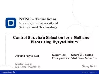
Control Structure Selection for a Methanol Plant using Hysys / Unisim. Supervisor: Sigurd Skogestad Co-supervisor: Vladimiros Minasidis. Adriana Reyes Lúa. Master Project Mid-Term Presentation. Spring 2014. Mid-term Presentation. Outline. Introduction Previous work

E N D
Control Structure Selection for a Methanol Plant using Hysys/Unisim Supervisor: SigurdSkogestad Co-supervisor: VladimirosMinasidis Adriana Reyes Lúa Master Project Mid-Term Presentation Spring 2014 Mid-term Presentation
Outline • Introduction • Previous work • Specialization Project • Work in progress • Future work
Plantwide Control • “Control structure design for complete chemical plants” • Systematic procedure for the design of an control structure, based on steady state plant economics. • Top down • Bottom up
Plantwide Control 1. Top-down Step 1: Define operational objectives (economics) and constraints. Step 2: Identify steady state degrees of freedom and determine steady state operation conditions. Step 3: Identify candidate measurements y and select CV1 =Hy Step 4: Select the location of the throughput manipulator.
Plantwide Control: The Challenge • To be accepted and used in industry, the procedure: • must result in processes with near optimal operation. • should not employ complex control technology. • simple to apply. • Proposed solution: • self-optimizing control. • automate procedure and hide complexities. • Can this be done using process simulators? • Intuitive. • Widely used. • Pre-loaded information. • Design mode vs. operation mode. • Poor numerical properties. • Not standardized.
Objective To investigate if commercial process simulators could be effectively used for the automation of the plantwide control procedure.
Case Study: Methanol Plant First of all, you need a model! Reactor, a separator, and a recycle stream with purge. Scheme of a methanol plant (Løvik,2001)
The Model The “operation mode” process simulation is the model. • Whenusingthistype of model: • Theinteractionsamongthe variables are notexplicit. • We do nothaveequationsto describe ourmodel.
Plantwide Procedure: Step 1 Define: Operational objectives (economics) and constraints. • Objectivefunctionforspecializationproject: • Reviewedobjectivefunction: The purge is now treated as a product. The costs of the purge and electricity were also reviewed.
Plantwide Procedure: Step 2 • Identify steady state degrees of freedom.
Plantwide Procedure: Step 2 • Identify steady state degrees of freedom. 4 steady state degrees of freedom. • Identify important disturbances. • Determine steady state operation conditions. You need to optimize!
Optimizing the Simulation As done for the Specialization Project COM Matlab UniSim • NLP Solver • fmincon • Interior point • (satisfies bounds) • NLP Model NLP model independent of NLP solver.
Plantwide Procedure: Step 2 Purge treated as waste (you pay for purging). Purge treated as product. Pressure (l), temperature (h), flow to compressor (l) Pressure (l), temperature (h), flow to compressor (l), UA slack (h)
Plantwide Procedure: Step 2 Pressure (l), temperature (h), flow to compressor (l) Pressure (l), temperature (h), flow to compressor (l), UA slack (h) • Noisymodel • Crudeareaapproximation • Control structurefor a single point. • stepsizeissues. • finergrid. • single region-wide control structure.
Gradient-based approach to solve the problem: • For each iteration step it does 2*n+1function evaluations. • Each iteration is expensive. • Dependant on step size. • Each function evaluation means running the simulation. • For the case study (6 variables), at least abt. 300 function evaluations are required. You want to reduce the number of function evaluations!
Derivative-free optimization • Objective function values available. • F is a “black box” that returns the value F(x) for any feasible x. • Derivative information: unavailable, unreliable, unpractical. • The function is expensive to evaluate or noisy. • Some algorithms can handle bounds a ≤ x ≤ b Same characteristics as our model.
Derivative-free optimization • Classification of algorithms: • Direct: search direction defined by computing values of the function directly. • Model based: construct a surrogate model of the function to guide the search process. • Local/Global: search domain definition. • Stochastic/Deterministic:random search steps or not.
Derivative-free trust- region methods • Surrogate and easy to evaluate model. • Obtained by interpolation. • Basic idea: • Define a region in which the model is an adequate representation of the objective function. • Choose the step (direction and length) to be the approximate minimizer of the model in this region.
Trust- region methods • Contours of a nonlinear function in a trust region. linear model quadratic model Conn, Andrew R., Scheinberg, Katya, Vicente, Luis N. IntroductiontoDerivative-Free Optimization, 2009
Trust- region algorithm 0. Initialize Solve trust region problem: calculate step Acceptance of step. Update model. Update trust region. Stopping criterion Quadratic model Real function Taylor approximation
Derivative-free trust- region algorithm • Theobjectivefunctionisapproximatedbyquadraticmodelsobtainedby a 2ndorder Taylor approximation. • Solves bound constrained optimization problems. • Considers bounds when calculating the trust region step. • Obtains an approximate solution for the approximation mk (xk + s) • The solution is in the intersection of the trust-region with the bound constraints.
Derivative-free trust- region algorithm • Derivative-free trust-regionalgorithm. • Theobjectivefunctionisapproximatedbyquadraticmodelsobtainedby a 2ndorder Taylor approximation. • Solves bound constrained optimization problems. • The number of interpolation points can vary. • In eachiteration, onlyoneinterpolationpointisreplaced • Theobjectivefunctionisevaluatedonceper iteration.
Derivative-free trust- region algorithm • Initialize: generate interpolation points and model. • Solve quadratic trust-region problem. • Acceptance test for the step. • Update trust-region radius • Alternative iteration • Re-calculate s in order to improve the geometry of the interpolation set. • Update interpolation set and quadratic model. • Stopping criterion.
Work to do • Finishprogrammingthe DFO algorithm. • Obtain more detailed active constraintregions. • Find control structures for the identified regions. • Investigate the posibility of finding a region-wide control structure.