Alignment scoring matrices and evolution
Alignment scoring matrices and evolution. ORF Graphs: types of edges. ATG TAG (single exon gene) ATG GT (initial coding exon) GT AG (intron) AG GT (internal exon) AG TAG (terminal coding exon) TAG ATG (intergenic region). Conceptual framework for
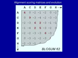

Alignment scoring matrices and evolution
E N D
Presentation Transcript
ORF Graphs: types of edges ATG TAG (single exon gene) ATG GT (initial coding exon) GT AG (intron) AG GT (internal exon) AG TAG (terminal coding exon) TAG ATG (intergenic region)
Conceptual framework for gene finding with ORF graphs Given an input sequence S, compute the ORF graph G for S. Score the vertices and edges in G using some scoring strategy or function, f. Extract the highest-scoring valid parse from G according to f.
Common assumptions • No overlapping genes • reasonably safe • No nested genes • reasonably safe • No partial genes • limiting; needs to be relaxed for real gene finders
Common assumptions (continued) • No non-canonical splice sites or start codons • GTG, TTG common start sites in bacteria • GC-AG and AT-AC introns present in plants and animals • No frame shifts or sequencing errors • OK for finished sequence
Common assumptions (continued) • Optimal parse only • useful, but if we allow the gene finder more guesses it may do better • Constraints on exon/intron lengths • max sizes needed for practical reasons • but, human introns can be >100,000 bp • for now we just miss those
Common assumptions (continued) • No split start/stop codons • introns can occur right in the middle of an ATG or TAG/TGA/TAA! • (most of) today’s gene finders will miss these • No alternative splicing • some species have an average of 2 alternative splicing products per gene • researchers actively working on this
Common assumptions (continued) • No selenocysteine codons • encoded by TGA • No ambiguity codes • R = purine = A or G • Y = pyrimidine = C or T • other codes for all possible ambiguous base calls
The (Eukaryotic) Gene Prediction Problem exons ATG…..GT…..AG…………GT….AG……..TAG UTR UTR introns Gene prediction is the problem of parsing a sequence into nonoverlapping coding segments(CDSs) consisting of exons separated by introns. Untranslated regions(UTR) are rarely predicted. This parsing problem can be visualized as one of choosing the best path through the graph of all open reading frames(ORFs): slide courtesy of Bill Majoros
Some Eukaryotic Gene-finding Programs gray boxes = developed in Salzberg lab slide courtesy of Bill Majoros
Similarities Between Gene-finding Programs GeneZilla GenScan Phat SNAP GlimmerHMM Augustus Genie Exonomy Unveil HMMgene VEIL Jigsaw Ensembl GAZE GHMMs HMMs Combiners TWAIN SLAM TWINSCAN GenomeScan DoubleScan SGP-1 SGP-2 GlimmerM Grail GrailEXP MORGAN GeneMark FGenesH ad hoc Homology-based slide courtesy of Bill Majoros
Gene Finding Strategies Gene finding programs can be classified into several types: (1) ad hoc. These apply an ad hoc scoring function to the set of all ORFs and then predict only those ORFs scoring above a predefined threshold. Examples are GRAIL and GlimmerM. (2) probabilistic. These adopt a rigorous probabilistic model of sequence structure and choose the most probable parse according to that probabilistic model. Examples are GenScan and GeneZilla. (3) homology-based. These utilize evidence in the form of homology. These can be either ad hoc (eg., GrailEXP) or probabilistic (eg., TwinScan, Slam, Twain). (4) combiners. These combine multiple forms of evidence, such as the predictions of other gene finders, and use ad hoc methods to arrive at a consensus prediction. Examples include Ewan Birney’s Ensembl and Jonathan Allen’s JIGSAW. slide courtesy of Bill Majoros
P(x) denotes the probability of event x occurring. P(x)=0.25 means, for example, that x occurs 25% of the time. P(x)=1 implies that the event x is certain to occur. P(x)=0 implies that x cannot occur. The probability of events x and y both occurring is denoted by: P(x, y) or P(x y) P(x | y) denotes the probability of event x occurring, given that y has occurred, or given that y is a true statement. If P(y)≠0 then: P(x | y) = P(x, y) / P(y) so that: P(x, y) = P(x | y) × P(y) If x and y are independent then: P(x, y) = P(x) × P(y), P(x | y) = P(x). Review of Probability Theory (joint probability) (conditional probability) (multiplication rule) (independence) slide courtesy of Bill Majoros
If x and y are mutually exclusive (i.e., can’t both happen), then: P(xy) = P(x) + P(y). If an experiment is guaranteed to yield one of a set of mutually exclusive events {x1,x2,…,xn} then Σ P(xi) = 1 If a set of events {x1,x2,…,xn} are all pairwise mutually independent then: P(x1, x2, …, xn) = Π P(xi) PM(x)=P(x|M) is an estimate of P(x) according to model M. Review of Probability Theory (the addition rule) n (partitioning rule) i=1 n (independence) i=1 (prob. model) slide courtesy of Bill Majoros
Ab initio Gene Finding = Modeling • Computational gene prediction is generally carried out as follows: • We formulate a mathematical model M which describes some method for generating DNA sequences and their gene structures. That is, M generates pairs of the form (S, ) for sequence S and gene structure . • 2. Using a set T of known genes, we customize or “train” the model so that the sequences and gene structures which M generates have the same statistical properties as the real genes in T. • 3. Given an un-annotated sequence S, we pretend that M generated S, even though we know that it did not. (Evolution and the cellular machinery generated it, not our model!) • 4. Since we assume that M generated S, we can determine precisely howlikely it is for M to have generated it—i.e., the precise intron/exon boundaries that M would have imposed while it was generating S. slide courtesy of Bill Majoros
A Model Generates Sequences and Gene Structures The underlying model of a gene finder generates both sequences and their gene structures. These can be denoted as pairs of the form (S,) for sequence S and gene structure . gene structure M exon 1 exon 2 exon 3 AGCTAGCAGTCGATCATGGCATTATCGGCCGTAGTACGTAGCAGTAGCTAGTAGCAGTCGATAGTA sequence slide courtesy of Bill Majoros
The Model Parameters Affect the Model’s Output The parameters to M determine the statistical properties of the sequences and gene models which it generates (both the structural properties of the gene models and frequences of individual bases). M AGCTAGCAGTCGATCATGGCATTATCGGCCGTAGTACGTAGCAGTAGCTAGTAGCAGTCGATAGTA 6,23,843,924… M TAGGCTCTATTAGCGCTATGCTACGTTATATTCTGATGTGTGATCGTATCTATATATCGATCTAGG 45,2,8214,32… M CCCTATCGCGCGCGCGCTATCACACACACTACGCGTCATTATCTTACTGAGCGCGCGCTATCGTAT 11,413,7,235,8… slide courtesy of Bill Majoros
Tuning the Model to Obtain Optimal Behavior The parameters to M can be tuned to make its outputs most similar to the set of known genes: known predicted AGCTAGCAGTCGATCATGGCATTATCGGCCGTAGTACGTAGCAGTAGCTAGTAGCAGTCGATAGTA M CGCGCTATCGATCGATCATCTGCGATCGTATATGCTACGGTCGTAGCTAGCTGATCGATCGATCGC 6,23,843,924… modify parms Still dissimilar AGCTAGCAGTCGATCATGGCATTATCGGCCGTAGTACGTAGCAGTAGCTAGTAGCAGTCGATAGTA M TGCTGCTATATGCTACGAGCATCTAGCTGACTTATCGCGCGCTAGCTAGCATCGATCGATCTAGCG 45,2,8214,32… modify parms AGCTAGCAGTCGATCATGGCATTATCGGCCGTAGTACGTAGCAGTAGCTAGTAGCAGTCGATAGTA similar M AGCTTTCAGTCGATCCCGGCATTATCGGCCGTAGCCCGTAGGGGTAGCTAGTACGCATCGATAGTA 11,413,7,235,8… slide courtesy of Bill Majoros
Using the Model to Predict Gene Structure Given an input sequence, we can ask what gene structure the model is most likely to have generated at the same time that it generated that sequence: parameter file sequence S 11,413,7,235,8… AGCTAGTACG… Suppose M was invoked 1,000,000,000,000,000,000 times. Collect those pairs (Si,i) where Si=S. Among those pairs, which gene structure is most common? Emit that . M (Si,i) Gene Finder XYZ (maximum a posteriori, MAP) gene structure slide courtesy of Bill Majoros