Spectroscopy with PACS
M82 PACS line imaging from the SHINING team ( Contursi et al. 2010 First Results workshop talk). Spectroscopy with PACS. Phil Appleton and Dario Fadda for the PACS Team. Important Resources. http:// nhscsci.ipac.caltech.edu. NHSC Proposal Planning Page

Spectroscopy with PACS
E N D
Presentation Transcript
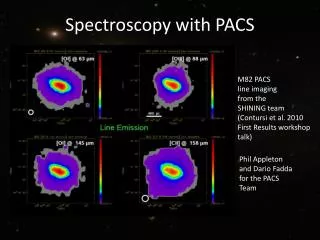
M82 PACS line imaging from the SHINING team (Contursi et al. 2010 First Results workshop talk) Spectroscopy with PACS Phil Appleton and Dario Fadda for the PACS Team
Important Resources http://nhscsci.ipac.caltech.edu • NHSC Proposal Planning Page https://nhscsci.ipac.caltech.edu/sc/index.php/ObservationPlanning/HomePage • NHSC HELPDESK • links to AOT Release notes for each spectrometer mode—very useful. • links to HSpot and Observer Manuals • links to other calibration documents
Line Spectroscopy • Chop/Nodding (Phil Appleton will discuss) • Chop rapidly between two sky position • Targeted “Line” scans or broad “Range/SED” spectroscopy available • Single Pointed ormapping on scale < 4 arcmins • Unchopped scans with “off” position (Dario Fadda will discuss) • Allows for targets that cannot be chopped • Line-scans or Range/SED Spectroscopy • Single pointed or mapping on any scale
Simple LINE SCAN– GRATING SCANS OVER TARGETED LINE ONLY Chop/Nod Cycle Each line is visited with one up and down scan per repetition Example above shows three lines in simple NodA/Nod B pattern
Range Scan • User can specify the range of the scan • Useful for known broad or multiple lines • Special version is SED mode where Blue/Red or Green Red bands scanned • Range Scan is only mode that allows exploitation of extended second order (see next slide) Range scans can provide broader coverage if there are multiple features User can control the scan range
Order Selection and Line/AOR You can only select in any one AOR either the 2nd or 3rd order paired with 1st order 3rd Either “Blue/RED” or “Green/RED” You can select multiple lines per AOR—for each line scanned you will get “for free” an observation in the blue or red band (e. g. If request 2nd/1st ordermodes and you observe [CII]158mm, you wlll “simultaneously” get “blue” observation at 158/2 = 79mm 2nd 1st is always selected Accessible in range/SED mode You can observe the same line 10 times (10 repetitions) or 5 different lines x 2 repetitions, or as many repetition-lines not exceeding 10 total per AOR. To repeat the whole sequence you can add more cycles. Note that calibration block is run at beginning or AOR.
For True Point Source • Know your position well! Place target at center array and use “Pointed Mode”. Be careful of any avoidance angle constraints (visualize in HSpot) • Be aware of distortions (rotation) in footprint of NODA and NOD B –only fully aligned at center of field
Chopped distortion on Large Throw(1, 3, 6 arcmin throw separations) Only the central few pixels are properly aligned for largest (LARGE) chopped throw. Best to use small or medium throw if possible. If you suspect your source is not a point-source or you are very unsure of its position to 1-2”, probably best NOT to use POINTED mode, but a fully sample mapping mode.
Mapping Slightly Extended SourcesChop-Nod Observations • First select target • Choose which “blue” order? 3rd+1st or 2nd+1st Note that if you have target lines in all three orders you will need 2 separate AORs • Choose a line (manual or from list) –don’t forget to check the box at right! • Enter continuum and line flux—saturation will trigger different capacitance—warning in Pacs time est. message • Select the Observational Mode • Set up the mapping parameters • raster step sizes (follow guidelines of the release )herschel.esac.esa.int/AOTsReleaseStatus.shtml )
Time estimation and S/N calculation”Also warnings for saturation a b c = a+b+c On slew IF ENTERED FLUX TOO LARGE: HSPOT WILL REQUEST A NEW GAIN BY CHANGING CAPACITANCE USUALLY FOR VERY HIGH FLUX > 10^4 Jy! (See PACS Observer Manual)
Cycles versus Repetitions versuscomplete AOR? • One line observation involves a complete up and down scan with the grating—this is called a repetition. 2 repetitions= 2 complete up and down scans • If you have one weak line (say [NII]205mm) and one strong one [CII]158mm, you can increase the number of repetitions on the [NII] line at the expense of the brighter line. e. g. 9 reps [NII], and say 1 rep for [CII]. If you need more time on both lines you can then increase the number of cycles. (complete sets of repetitions). A cycle does NOT lead to a repeat of the calibration block. If you request a new AOR you will allows get a new cal block.
Repetition v Cycles: large-chopHSpot v5.0.2 (from obs estimate button) • C/N Single pointing mode 1 line, 2 repetitons Total time = 952s (on source*=688s, cal=129s) • C/N Single pointing 1 line, 2 cycles Total time = 985s (on source 688s) Extra inst. overhead of 33s! • C/N Single pointing 1 line, 1 rep, 2 AORs Total time = 2 x 586 (on 688s; cal=2 x 129) = 1172s but you get 2 cal blocks..very inefficient.. Repetitions have less overhead than cycles. * Note HSpot reports “On source” time including the time chopped off!
Some considerations withChop-Nod • Is your source point-like, slightly extended or very extended, or HUGE? (If huge use unchopped scan mode) • Choose an appropriate chopper throw small=±0.5 medium =±1.5 large =±3 arcmins • Choose the right mapping strategy for your object (Pointed = point source, large-scale map or small map use correct raster step size) • Nyquist spatial sampling is best achieved in instrument coordinates rather than sky coordinates. Coverage can be less uniform in sky coordinates because of potential telescope pointing drifts • If you want to ratio two lines, best include in same AOR to ensure pixels fall on same place on sky
Worked Examples: (AOR Design one or more AOR which provides minimal coverage along major axis of NGC 4565 Map along the major axis of the galaxy NGC 4565 in [OI]63um line with 5 x 2 raster map-covering with 38 x 38 tile size” redshiftz = 0.004 (CHOP-NOD)—left below right below—an unchopped scan—see DARIO detector cords Off position z y Unchopped scan can be programmed in sky coords Chop-nod mapping is limited to instrument plane (chops along z axis). Limited ability to map a feature without multiple AORs = 4.1hrs 3 x (38 x 38” 5 x 2 raster) one line Unchopped grating scan in RA/Dec Coords. 38 x 38 “ 20 x 2 raster at orientation = 135 degrees = 3.7 hrs clock time