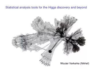
Statistical analysis tools for the Higgs discovery and beyond
670 likes | 901 Vues
Statistical analysis tools for the Higgs discovery and beyond. Wouter Verkerke (Nikhef). What do you want to know?. Physics questions we have… Does the (SM) Higgs boson exist? What is its production cross-section? What is its boson mass ?

Statistical analysis tools for the Higgs discovery and beyond
E N D
Presentation Transcript
Statistical analysis tools for the Higgs discovery and beyond Wouter Verkerke (Nikhef)
What do you want to know? • Physics questions we have… • Does the (SM) Higgs boson exist? • What is its production cross-section? • What is its boson mass? • Statistical tests constructprobabilistic statements:p(theo|data), or p(data|theo) • Hypothesis testing (discovery) • (Confidence) intervalsMeasurements & uncertainties • Result: Decision based on tests “As a layman I would now say: I think we have it” Wouter Verkerke, NIKHEF
All experimental results start with the formulation of a model • Examples of HEP physics models being tested • SM with m(top)=172,173,174 GeV Measurement top quark mass • SM with/without Higgs boson Discovery of Higgs boson • SM with composite fermions/Higgs Measurement of Higgs coupling properties • Via chain of physics simulation, showering MC, detector simulation and analysis software, a physics model is reduced to a statistical model Wouter Verkerke, NIKHEF
The HEP analysis workflow illustrated LHC data Simulation of ATLASdetector Simulation of ‘soft physics’physics process Simulation of high-energyphysics process P(m4l|SM[mH]) Reconstruction of ATLAS detector Observed m4l Analysis Event selection prob(data|SM) Wouter Verkerke, NIKHEF Wouter Verkerke, NIKHEF
All experimental results start with the formulation of a model • Examples of HEP physics models being tested • SM with m(top)=172,173,174 GeV Measurement top quark mass • SM with/without Higgs boson Discovery of Higgs boson • SM with composite fermions/Higgs Measurement of Higgs coupling properties • Via chain of physics simulation, showering MC, detector simulation and analysis software, a physics model is reduced to a statistical model • A statistical model defines p(data|theory) for all observable outcomes • Example of a statistical model for a counting measurement with a known background s=0 s=5 s=10 s=15 NB: b is a constant in this example Definition: the Likelihood is P(observed data|theory) Nobs Wouter Verkerke, NIKHEF
Everything starts with the likelihood • All fundamental statistical procedures are based on the likelihood function as ‘description of the measurement’ Nobs e.g. L(15|s=0) e.g. L(15|s=10) Frequentist statistics Bayesian statistics Maximum Likelihood Confidence interval on s Posterior on s s = x ± y
Everything starts with the likelihood Frequentist statistics Bayesian statistics Maximum Likelihood Confidence intervalor p-value Posterior on sor Bayes factor s = x ± y Wouter Verkerke, NIKHEF
How is Higgs discovery different from a simple fit? Gaussian + polynomial Higgs combination model ROOT TF1 ROOT TH1 “inside ROOT” MLestimation ofparameters μ,θ using MINUIT (MIGRAD, HESSE, MINOS) μ = 5.3 ± 1.7 Wouter Verkerke, NIKHEF
How is Higgs discovery different from a simple fit? Likelihood Modelorders of magnitude morecomplicated. Describes - O(100) signal distributions - O(100) control sample distr. - O(1000) parameters representing syst. uncertainties Gaussian + polynomial Higgs combination model ROOT TF1 ROOT TH1 “inside ROOT” MLestimation ofparameters μ,θ using MINUIT (MIGRAD, HESSE, MINOS) Frequentist confidence intervalconstruction and/or p-valuecalculation not availableas ‘ready-to-run’ algorithm in ROOT μ = 5.3 ± 1.7 Wouter Verkerke, NIKHEF
How is Higgs discovery different from a simple fit? Gaussian + polynomial Higgs combination model Model Building phase (formulation of L(x|H) ROOT TF1 ROOT TH1 “inside ROOT” MLestimation ofparameters μ,θ using MINUIT (MIGRAD, HESSE, MINOS) μ = 5.3 ± 1.7 Wouter Verkerke, NIKHEF
How is Higgs discovery different from a simple fit? Gaussian + polynomial Higgs combination model ROOT TF1 ROOT TH1 “inside ROOT” MLestimation ofparameters μ,θ using MINUIT (MIGRAD, HESSE, MINOS) μ = 5.3 ± 1.7 Model Usage phase (use L(x|H) to make statement on H) Wouter Verkerke, NIKHEF
How is Higgs discovery different from a simple fit? Gaussian + polynomial Higgs combination model Design goal: Separate buildingof Likelihood model as much as possiblefrom statistical analysis using the Likelihood model • More modular software design • ‘Plug-and-play with statistical techniques • Factorizes work in collaborative effort ROOT TF1 ROOT TH1 “inside ROOT” MLestimation ofparameters μ,θ using MINUIT (MIGRAD, HESSE, MINOS) μ = 5.3 ± 1.7 Wouter Verkerke, NIKHEF
The idea behind the design of RooFit/RooStats/HistFactory • Modularity, Generality and flexibility • Step 1 – Construct the likelihood function L(x|p) • Step 2 – Statistical tests on parameter of interest p Procedure can be Bayesian, Frequentist, or Hybrid), but always based on L(x|p) • Steps 1 and 2 are conceptually separated, and in Roo* suit also implemented separately. RooFit, or RooFit+HistFactory RooStats Wouter Verkerke, NIKHEF
The idea behind the design of RooFit/RooStats/HistFactory • Steps 1 and 2 can be ‘physically’ separated (in time, or user) • Step 1 – Construct the likelihood function L(x|p) • Step 2 – Statistical tests on parameter of interest p RooFit, or RooFit+HistFactory Complete descriptionof likelihood model,persistable in ROOT file (RooFit pdf function) Allows full introspectionand a-posteriori editing RooWorkspace RooStats Wouter Verkerke, NIKHEF
The benefits of modularity • Perform different statistical test on exactly the same model RooFit, or RooFit+HistFactory RooWorkspace RooStats (Frequentistwith toys) RooStats BayesianMCMC “Simple fit” RooStats (Frequentistasymptotic) (ML Fit withHESSE orMINOS) Wouter Verkerke, NIKHEF
RooFit WV + D. Kirkby- 1999
RooFit – Focus: coding a probability density function • Focus on one practical aspect of many data analysis in HEP: How do you formulate your p.d.f. in ROOT • For ‘simple’ problems (gauss, polynomial) this is easy • But if you want to do unbinned ML fits, use non-trivial functions, or work with multidimensional functions you quickly find that you need some tools to help you • The RooFit project started in 1999 for data modeling needs for BaBar collaboration initially, publicly available in ROOT since 2003
RooFit core design philosophy • Mathematical objects are represented as C++ objects Mathematical concept RooFit class variable RooRealVar function RooAbsReal PDF RooAbsPdf space point RooArgSet integral RooRealIntegral list of space points RooAbsData Wouter Verkerke, NIKHEF
Data modeling – Constructing composite objects • Straightforward correlation between mathematical representation of formula and RooFit code Math RooGaussian g RooFit diagram RooRealVar x RooRealVar m RooFormulaVar sqrts RooRealVar s RooFit code RooRealVar x(“x”,”x”,-10,10) ; RooRealVar m(“m”,”mean”,0) ; RooRealVar s(“s”,”sigma”,2,0,10) ; RooFormulaVar sqrts(“sqrts”,”sqrt(s)”,s) ; RooGaussian g(“g”,”gauss”,x,m,sqrts) ; Wouter Verkerke, NIKHEF
New feature for LHC RooFit core design philosophy • A special container class owns all objects that together build a likelihood function Gauss(x,μ,σ) Math RooWorkspace (keeps all parts together) RooGaussiang RooFit diagram RooRealVar x RooRealVarm RooRealVars RooFit code RooRealVarx(“x”,”x”,-10,10) ; RooRealVarm(“m”,”y”,0,-10,10) ; RooRealVars(“s”,”z”,3,0.1,10) ; RooGaussiang(“g”,”g”,x,m,s) ; RooWorkspace w(“w”) ;w.import(g) ; Wouter Verkerke, NIKHEF
Populating a workspace the easy way – “the factory” • The factory allows to fill a workspace with pdfs and variables using a simplified scripting language Gauss(x,μ,σ) Math New feature for LHC RooWorkspace RooAbsReal f RooFit diagram RooRealVar x RooRealVar y RooRealVar z RooFit code RooWorkspace w(“w”) ; w.factory(“Gaussian::g(x[-10,10],m[-10,10],z[3,0.1,10])”);
Model building – (Re)using standard components • RooFit provides a collection of compiled standard PDF classes RooBMixDecay Physics inspired ARGUS,Crystal Ball, Breit-Wigner, Voigtian,B/D-Decay,…. RooPolynomial RooHistPdf Non-parametric Histogram, KEYS RooArgusBG RooGaussian Basic Gaussian, Exponential, Polynomial,…Chebychev polynomial Easy to extend the library: each p.d.f. is a separate C++ class Wouter Verkerke, NIKHEF
g(x;m,s) m(y;a0,a1) Model building – (Re)using standard components • Library p.d.f.s can be adjusted on the fly. • Just plug in any function expression you like as input variable • Works universally, even for classes you write yourself • Maximum flexibility of library shapes keeps library small g(x,y;a0,a1,s) RooPolyVar m(“m”,y,RooArgList(a0,a1)) ; RooGaussian g(“g”,”gauss”,x,m,s) ; Wouter Verkerke, NIKHEF
From empirical probability models to simulation-based models • Large difference between B-physics and LHC hadron physics is that for the latter distributions usually don’t follow simple analytical shapes • But concept of simulation-driven template models can also extent to systematic uncertainties. Instead of empirically chosen ‘nuisance parameters’ (e.g. polynomial coefs) construct degrees of freedom that correspond to known systematic uncertainties Unbinned analytical probability model (Geant) Simulation-drivenbinned template model Wouter Verkerke, NIKHEF
The HEP analysis workflow illustrated LHC data Simulation of ATLASdetector Simulation of ‘soft physics’physics process Detectormodellinguncertainties Soft Theoryuncertainties Simulation of high-energyphysics process Hard Theoryuncertainties P(m4l|SM[mH]) Reconstruction of ATLAS detector Observed m4l Analysis Event selection prob(data|SM) Wouter Verkerke, NIKHEF Wouter Verkerke, NIKHEF
Modeling of shape systematics in the likelihood • Effect of any systematic uncertainty that affects the shape of a distribution can in principle be obtained from MC simulation chain • Obtain histogram templates for distributions at ‘+1σ’ and ‘-1σ’ settings ofsystematic effect • Challenge: construct an empirical response function based on the interpolation of the shapes of these three templates. “Jet Energy Scale” ‘-1σ’ ‘nominal’ ‘+1σ’ Wouter Verkerke, NIKHEF
Need to interpolate between template models • Need to define ‘morphing’ algorithm to define distribution s(x) for each value of α s(x)|α=+1 s(x)|α=0 s(x,α=+1) s(x)|α=-1 s(x,α=0) s(x,α=-1) WouterVerkerke, NIKHEF
Visualization of bin-by-bin linear interpolation of distribution α x Wouter Verkerke, NIKHEF
Example 2 : binned L withsyst • Example of template morphingsystematic in a binnedlikelihood // Import template histograms in workspace w.import(hs_0,hs_p,hs_m) ; // Construct template models from histograms w.factory(“HistFunc::s_0(x[80,100],hs_0)”) ; w.factory(“HistFunc::s_p(x,hs_p)”) ; w.factory(“HistFunc::s_m(x,hs_m)”) ; // Construct morphing model w.factory(“PiecewiseInterpolation::sig(s_0,s_,m,s_p,alpha[-5,5])”) ; // Construct full model w.factory(“PROD::model(ASUM(sig,bkg,f[0,1]),Gaussian(0,alpha,1))”) ; Wouter Verkerke, NIKHEF
Other uncertainties in MC shapes – finite MC statistics • In practice, MC distributions used for template fits have finite statistics. • Limited MC statistics represent an uncertainty on your model how to model this effect in the Likelihood? Wouter Verkerke, NIKHEF
Other uncertainties in MC shapes – finite MC statistics • Modeling MC uncertainties: each MC bin has a Poisson uncertainty • Thus, apply usual ‘systematics modeling’ prescription. • For a single bin – exactly like original counting measurement Fixed signal, bkg MC prediction Signal, bkgMC nuisance params Subsidiary measurement for signal MC(‘measures’ MC prediction si with Poisson uncertainty)
Code example – Beeston-Barlow • Beeston-Barlow-(lite) modelingof MC statisticaluncertainties // Import template histogram in workspace w.import(hs) ; // Construct parametric template models from histograms// implicitly creates vector of gamma parameters w.factory(“ParamHistFunc::s(hs)”) ; // Product of subsidiary measurement w.factory(“HistConstraint::subs(s)”) ; // Construct full model w.factory(“PROD::model(s,subs)”) ; Wouter Verkerke, NIKHEF
Code example: BB + morphing • Template morphing modelwith Beeston-Barlow-liteMC statistical uncertainties // Construct parametric template morphing signal model w.factory(“ParamHistFunc::s_p(hs_p)”) ; w.factory(“HistFunc::s_m(x,hs_m)”) ; w.factory(“HistFunc::s_0(x[80,100],hs_0)”) ; w.factory(“PiecewiseInterpolation::sig(s_0,s_,m,s_p,alpha[-5,5])”) ; // Construct parametric background model (sharing gamma’s with s_p) w.factory(“ParamHistFunc::bkg(hb,s_p)”) ; // Construct full model with BB-lite MC stats modeling w.factory(“PROD::model(ASUM(sig,bkg,f[0,1]),HistConstraint({s_0,bkg}),Gaussian(0,alpha,1))”) ;
The structure of an (Higgs) profile likelihood function • Likelihood describing Higgs samples have following structure Signal region 1 ‘Constraint θn’ Strength ofsystematic uncertainties Signal region 2 ‘Constraint θ1’ ‘Constraint θn’ Control region 1 Control region 2 Wouter Verkerke, NIKHEF
The structure of an (Higgs) profile likelihood function • A simultaneous fit of physics samples and (simplified) performance measurements ‘Subsidiary measurement n’Factorization scale Signal region 1 ‘Simplified Likelihoodof a measurement relatedto systematic uncertainties’ Signal region 2 ‘Subsidiary measurement 1’ ‘Jet Energy scale’ ‘Subsidiary measurement 2’ B-tagging eff Control region 1 Control region 2 Wouter Verkerke, NIKHEF
The workspace • The workspace concept has revolutionized the way people share and combine analysis • Completely factorizes process of building and using likelihood functions • You can give somebody an analytical likelihood of a (potentially very complex) physics analysis in a way to the easy-to-use, provides introspection, and is easy to modify. RooWorkspace w(“w”) ; w.import(sum) ; w.writeToFile(“model.root”) ; model.root RooWorkspace Wouter Verkerke, NIKHEF
Using a workspace // Resurrect model and data TFile f(“model.root”) ; RooWorkspace* w = f.Get(“w”) ; RooAbsPdf* model = w->pdf(“sum”) ; RooAbsData* data = w->data(“xxx”) ; // Use model and data model->fitTo(*data) ;RooPlot* frame = w->var(“dt”)->frame() ; data->plotOn(frame) ; model->plotOn(frame) ; RooWorkspace Wouter Verkerke, NIKHEF Wouter Verkerke, NIKHEF
The idea behind the design of RooFit/RooStats/HistFactory • Step 1 – Construct the likelihood function L(x|p) • Step 2 – Statistical tests on parameter of interest p RooWorkspace w(“w”) ; w.factory(“Gaussian::sig(x[-10,10],m[0],s[1])”) ; w.factory(“Chebychev::bkg(x,a1[-1,1])”) ; w.factory(“SUM::model(fsig[0,1]*sig,bkg)”) ; w.writeToFile(“L.root”) ; RooFit, or RooFit+HistFactory Complete descriptionof likelihood model,persistable in ROOT file (RooFit pdf function) Allows full introspectionand a-posteriori editing RooWorkspace RooWorkspace* w=TFile::Open(“L.root”)->Get(“w”) ; RooAbsPdf* model = w->pdf(“model”) ; pdf->fitTo(data) ; RooStats Wouter Verkerke, NIKHEF
Example RooFit component model for realistic Higgs analysis Likelihood model describing the ZZ invariant mass distribution including all possible systematic uncertainties RooFit workspace variables function objects Graphical illustration of functioncomponents that call each other
Analysis chain identical for highly complex (Higgs) models • Step 1 – Construct the likelihood function L(x|p) • Step 2 – Statistical tests on parameter of interest p Complete descriptionof likelihood model,persistable in ROOT file (RooFit pdf function) Allows full introspectionand a-posteriori editing RooWorkspace RooWorkspace* w=TFile::Open(“L.root”)->Get(“w”) ; RooAbsPdf* model = w->pdf(“model”) ; pdf->fitTo(data,GlobalObservables(w->set(“MC_GlObs”),Constrain(*w->st(“MC_NuisParams”) ; RooStats Wouter Verkerke, NIKHEF
Workspaces power collaborative statistical modelling • Ability to persist complete(*) Likelihood models has profound implications for HEP analysis workflow • (*) Describing signal regions, control regions, and including nuisance parameters for all systematic uncertainties) • Anyone with ROOT (and one ROOT file with a workspace) can re-run any entire statistical analysis out-of-the-box • About 5 lines of code are needed • Including estimate of systematic uncertainties • Unprecedented new possibilities for cross-checking results, in-depth checks of structure of analysis • Trivial to run variants of analysis (what if ‘Jet Energy Scale uncertainty’ is 7% instead of 4%). Just change number and rerun. • But can also make structural changes a posteri. For example, rerun with assumption that JES uncertainty in forward and barrel region of detector are 100% correlated instead of being uncorrelated. Wouter Verkerke, NIKHEF
Collaborative statistical modelling • As an experiment, you can effectively build a library of measurements, of which the full likelihood model is preserved for later use • Already done now, experiments have such libraries of workspace files, • Archived in AFS directories, or even in SVN…. • Version control of SVN, or numbering scheme in directories allows for easy validation and debugging as new features are added • Building of combined likelihood models greatly simplified. • Start from persisted components. No need to (re)build input components. • No need to know how individual components were built, or are internally structured. Just need to know meaning of parameters. • Combinations can be produced (much) later than original analyses. • Even analyses that were never originally intended to be combined with anything else can be included in joint likelihoods at a later time Wouter Verkerke, NIKHEF
Higgsdiscoverystrategy – addeverythingtogether HZZllll Hττ HWWμνjj +… Dedicated physics working groups define search for each of the major Higgs decay channels (HWW, HZZ, Hττetc).Output is physics paper or note, and a RooFit workspace with the full likelihood function Assume SM rates A small dedicated team of specialists builds a combined likelihood from the inputs. Major discussion point: naming of parameters, choice of parameters for systematic uncertainties (a physics issue, largely)
The benefits of modularity • Technically very straightforward to combine measurements RooFit, or RooFit+HistFactory RooWorkspace RooWorkspace Higgs channel 1 Higgs channel 2 Lightweightsoftware toolusing RooFiteditor tools(~500 LOC) Combiner Insertion of combination step does notmodify workflow before/after combination step Higgs Combination RooWorkspace RooStats RooStats Wouter Verkerke, NIKHEF
Workspace persistence of really complex models works too! Atlas Higgs combination model (23.000 functions, 1600 parameters) F(x,p) x p Model has ~23.000 function objects, ~1600 parameters Reading/writing of full model takes ~4 secondsROOT file with workspace is ~6 Mb
With these combined models the Higgs discovery plots were produced… LATLAS(μ,θ) = CMS Neymanconstructionwith profile likelihood ratiotest Wouter Verkerke, NIKHEF
More benefits of modularity • Technically very straightforward to reparametrize measurements RooFit, or RooFit+HistFactory StandardHiggs combination RooWorkspace Lightweightsoftware toolusing RooFiteditor tools Reparametrize Reparametrizationstep does notmodify workflow BSMHiggs combination RooWorkspace RooStats RooStats Wouter Verkerke, NIKHEF
Portal model (mX) BSM Higgs constraints fromreparametrization of SM HiggsLikelihood model Simplified MSSM (tanβ,mA) Two Higgs Double Model(tanβ,cos(α-β)) Imposter model(M,ε) Minimal composite Higgs(ξ) (ATLAS-CONF-2014-010) Wouter Verkerke, NIKHEF
An excursion – Collaborative analyses with workspaces • How can you reparametrize existing Higgs likelihoods in practice? • Write functions expressions corresponding to new parameterization • Import transformation in workspace, edit existing model w.factory(“expr::mu_gg_func(‘(KF2*Kg2)/ (0.75*KF2+0.25*KV2)’, KF2,Kg2,KV2) ; w.import(mu_gg_func) ; w.factory(“EDIT::newmodel(model,mu_gg=mu_gg_gunc)”) ; Wouter Verkerke, NIKHEF